2 Pipeline Design for Deep Water
2.1 Introduction
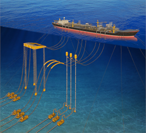
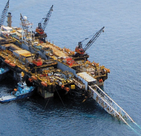
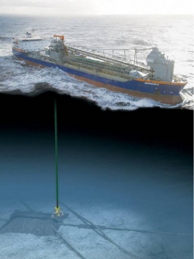
A typical deepwater pipeline system is designed to transport produced fluids from several subsea wells directly or through a subsea manifold on to the floating production system via pipelines and risers. In addition to the production pipeline system, there are:
export lines to export gas and/or oil to shore or offloading buoy.
water (or gas) injection lines to inject water (or gas) from topside to well,
service lines for service oil circulation,
chemical lines for chemical injection into production lines,
gas lift lines for gas injection into production lines.
![[Tip]](tip.png) | Tip Click these links below for access to 3D resources: |
Key components of the pipeline system are pipe, corrosion protection, field joint coating (FJC), terminations, spools, etc.
Pipelines are the most economical method for transporting large quantities of fluids on moderate distances. Other modes are more economical only when the quantities are too small to justify the capital cost of a pipeline or where technical difficulties make it impossible to construct a pipeline.
Principal technical difficulties for deepwater pipelines project are related to:
fluid properties
environmental at the site conditions: depth, seastate, current, sea-temp, soil properties, etc
pipeline routing and seabed configuration
pipeline properties (steel wall, grade, coating type, etc)
functional loading (internal pressure, slugging, fluid temp, pressure cycling, buckling, expansion, etc)
environmental loading (external pressure, VIV, drag, fatigue, etc)
accidental loading.
A pipeline is subject to different types of loads, the main loading on the pipeline system are:
functional loads
environmental loads
accidental loads
construction/installation loads
interference loads
and other
Refer to DNVGL ST F101 as guideline for definition and examples of loading.
A pipeline has to meet several design criteria. It has to be strong enough to resist internal pressure, which in force terms is usually much the largest load it has to carry and external pressure when depressurised. It has to be strong enough to withstand other loads applied during installation and operation, principally external pressure, bending, axial tension, torsion and shear. It may have to carry large concentrated loads applied by installation method. It has to be made out of materials which guarantee the life time of the pipeline under erosion and corrosion effects. It has to be heavy enough to be stable against hydrodynamic forces, but not so heavy that it sinks into the seabed or become over-stressed when it spans low points.
It would be wrong to suppose that all these questions become more severe when the pipe is in deep water. On some instances, many of them become easier. Usually, though not always, the currents near the bottom are quite small in deep water, because surface wave action is insignificant more than half a wavelength below the surface, and because tidal flows are insufficient to generate high velocities because of the large flow cross-section.
Most pipe-laying techniques lay the pipe with the internal atmospheric pressure. In deep water, the pipe wall is then subject to a net external hydrostatic pressure during installation. In operation, the pipe is subject to a net internal pressure and the depth and hence the external hydrostatic pressure may serve to reduce the required minimum burst wall thickness, particularly if the selected wall thickness includes a corrosion allowance which will be present during installation and consumed during operation.
The obvious difficulty is that external pressure may cause the pipeline to propagation buckling which is first initiated by a local buckling of the pipe wall due to external hydrostatic pressure, axial force and bending moment then runs along the pipe under the effect of external pressure, collapsing the pipe into a dumb-bell cross section. Buckle propagation could destroy many miles of pipeline. The determination of pipe wall thickness to mitigate the buckling problem is presented in Section 2.3, “Pipeline Design Method” .
Some deepwater pipelines are designed so that the maximum net external pressure is lower than the propagation pressure, so that propagation cannot possibly occur. This becomes an onerous requirement in deep water, and a less conservative approach is to install buckle arrestors, so that a buckle initiated by unexpectedly severe bending might propagate to the next arrester, but could not destroy the whole length. The calculation and design of buckle arrestors is a well known technique.
External pressure governs the design of pipelines conventionally installed in deep water. This condition is most severe during installation, when the pipelines carry demanding combination of external pressure, bending and tension.
2.2 Material Selection
The selection of a material for a pipeline is a compromise between optimum corrosion resistance, required mechanical properties, ‘fabricability’, availability and cost. It may often be the case that a final choice has to be made between two or more optional materials which may differ in the extent to which they meet all the desired service requirements for the anticipated required lifetime of the project.
Pipeline material selection is mainly driven by:
the type of the fluid and associated content (H2S, CO2, sand, etc.) that could significantly increase corrosion and erosion issues
functional requirements and field architecture,
pipeline operational philosophy (like operational pigging or inhibitors injection),
installation philosophy like reeling and plastic deformations, weldability
In the extreme cases where corrosion risks are either negligible or very severe, material selection is fairly simple and a typical choice will be carbon steel or corrosion resistant alloys respectively.
In the extreme cases where corrosion risks are either negligible or very severe, material selection is fairly simple and a typical choice will be carbon steel or corrosion resistant alloys respectively. Between these two extreme cases, the final choice of material may lie between carbon steel, with corrosion allowance and coating, cladding or inhibitor protection, or various corrosion resistant alloy options. In this situation, past practice may have been to select the option which requires the least upfront capital expenditure.
Increasingly, however, the selection of materials is being made not simply on what is immediately the cheapest technically acceptable option, but on a longer term view of the costs incurred for the duration of a project. The Life Cycle Costing (LCC) approach utilises established accounting methods to compare the costs of alternative materials selections by calculating the ‘’present day value’’ of future costs associated with the chosen materials. By using LCC it can often be demonstrated that paying out more at the start for corrosion resistant alloys rather than an apparently much cheaper material, results in substantial savings in operating, maintenance and repair costs in the future.
One of the key benefits of using LCC in a comprehensive way is that it obliges the user to take a global view of the issue in question and not to solve a single problem in isolation of all the other factors which are affected or may affect the decision making process. Each case has to be calculated separately taking into consideration the material dimensions, fabrication method and pipe laying rate for the different materials, oil/gas production rate, inhibitor or glycol injection rate for carbon steel, appropriate inspection methods and frequency, etc.
Details recommendations are provided in [35], which provide general principles, engineering guidance and requirements for material selection and corrosion protection for all parts of offshore installations:
Corrosion and material selection evaluations.
Specific material selection where appropriate.
Corrosion protection.
Design limitations for candidate materials.
Qualification requirements for new materials or new applications.
2.3 Pipeline Design Method
2.3.1 General Consideration
The pipeline design calculations aim to determine the pipeline characteristics, such as external diameter or wall thickness, which will allow it to withstand not only the requirements of the production phase (resistance to the internal pressure and corrosion, stability on the seabed despite the seabed current forces, etc.) but also the installation loads (external pressure if the pipe is installed air filled, bending and compression forces, tension, etc.).
In the past, pipeline design or rules were based on allowable stresses computed from the material Specified Minimum Yield Strength to which a usage factor is applied (typically from 0.7 - 0.9 depending on the load cases). The last few years have seen the introduction of reliability-based Limit State Design (LDS) for offshore pipeline; this is a radical change in design philosophy as its application is based on risk assessment and probabilistic approaches.
The relatively recent code [13] which is based on the Limit State Design, has been first used for the design of the many pipelines around the world.
Pipeline design is a key issue within the offshore oil & gas engineering disciplines. The following section aims to describe a typical pipeline design approach and its general philosophy based on the [13]: “Submarine Pipeline Systems”.
During the design phase, the following points will be checked out:
Pipe material selection (based on produced fluid chemistry)
Pipe diameter (based on required flow rate and pressure drops)
Pipe wall thickness
Internal pressure containment
Hydrostatic collapse
Local buckling
Buckling propagation
On-bottom stability check
Thermal design (flow assurance during steady and transient states)
Pipe expansion calculations (thermal expansion and pressure end-cap effect)
Global buckling (lateral and upheaval buckling)
Protection
Cathodic protection
Span calculations
Fatigue when suspended
Pipeline Walking
2.3.2 Pipeline Diameter Determination
General
The pipeline design codes do not specify the specific methodology or requirements for assessing pipeline diameter. Pipeline diameter is determined by assessing pressure loss for the design flow rate and balancing that with available pressure. It is normal practice to use standard API 5L diameters as this minimises availability issues associated with procurement of the line-pipe.
Standard flow simulation software, such as PIPESIM, is often used for assessing diameter requirements, although it is possible to perform hand calculations for single-phase oil or gas flow. The basic methods for calculation of pressure drop in single-phase flow are described in this section, and issues relating to diameter selection for multiphase lines are reviewed.
Pressure Drop in Liquid Lines
The basic principles for flow in a pipe are based on Bernoulli’s equation for conservation of energy in flow. This basically states that the summation of pressure energy, kinetic energy, potential energy, thermal energy and energy lost from the system at any point in the system is constant.
For liquid flow we assume that the fluid is incompressible and therefore velocity and kinetic energy are constant and can be ignored. We also assume that the thermal energy does not influence the flow characteristics and therefore we can treat thermal energy and heat loss separately. This leaves pressure, elevation and frictional losses.
The evaluation of pressure change due to elevation is straightforward. To evaluate the pressure drop due to frictional losses the Darcy equation as shown below is used.

This equation works for any combinations of compatible units.
- ρ is density
- V is flow velocity;
- L is pipeline length;
- D is pipeline internal diameter;
- f is friction factor, a function of Reynolds number and relative roughness.
Reynolds number is given by:
![]()
Where:
ν is kinematic viscosity.
The friction factor, f, can be derived from the Moody diagram. This plots friction factor against Reynolds number for a range of internal relative roughness. It should be noted that f is nearly constant in the turbulent region.
The relative internal roughness is defined as the absolute roughness, k divided by the internal diameter. Some typical values for k are shown below:
|
If a pipe is internally coated with FBE (e.g. water injection flow-line) the surface roughness improves dramatically, with the value for k dropping down to 0.005mm.
As an alternative to the Moody diagram, the following equations may be used for determining the friction factor, f. For turbulent flow (Re>2000), the Colebrook White equation may be used.
Pressure Drop in Gas Lines
In gas lines, the product is compressible and therefore density and velocity change as the gas flows through the pipeline. Whilst the assessment of diameter requirements is more complicated, and is often solved by the use of flow simulation software, there are empirical formulae available which enable hand calculations to be performed. The Weymouth and Panhandle (large diameter lines) equations are recommended for most cases.
Diameter for Multiphase Flow
Multiphase flow conditions can not be solved with hand calculations. Flow correlations have been developed for steady state multiphase flow, which define the flow regime within the pipe and the corresponding pressure losses. These correlations, such as Beggs and Brill, are used within software such as PIPESIM.
In sizing for multiphase flow, consideration has to be given to the flow regime in the pipeline and any implications that may have. One main issue is to avoid or at least control slugging flow as this can have major implications for process equipment sizing, fatigue, and pressure drop. Multiphase flow is generally associated with production flow-lines, driven by reservoir pressures. There can be significant differences in flow rates between start of life and end of life, and low flow rates at end of life can result in liquid hold-up and slugging flow. Issues/solutions to consider include:
|
The flow velocity needs to be considered. At high flow rates, solids or water droplets can start to cause erosion of the pipeline walls, particularly at bends. API RP 14E gives the empirical formula shown below for the velocity at which erosion may start to occur. Normal practice would be to ensure that this velocity is not exceeded:

The units are metric, with velocity Ve in m/s and density ρ in kg/m3.
Besides, the [31] is intended used instead of the [7]. [31] is a new Recommended Practice developed based on DNV’s long term experience within erosion in piping systems. The RP gives correlations for estimation of erosion in pipe bends, Tee-bends, welded joints, in contractions and in smooth pipes. The procedure is applicable both for dimensioning of pipe systems and for estimation of erosion in existing systems based on the production characteristics; i.e. gas and liquid flow rate, physical properties of gas and liquid, pipe dimensions, radius of curvature for the pipe bends, particle size and the particle concentrations/amount of produced particles.
2.3.3 Pipeline Wall Thickness
Introduction
The selection of the pipe wall thickness is one of the most important factors in the design process of a pipeline. The choice of the wall thickness has an immediate effect on the pipe design and installation load. The various criteria upon which the wall thickness is selected are discussed below in this section. This section also discusses the selection of wall thickness particularly for pipe-reeling method and deep water applications.
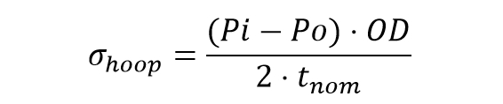
Internal Pressure
Wall thickness requirements for internal pressure are based on thin walled theory.
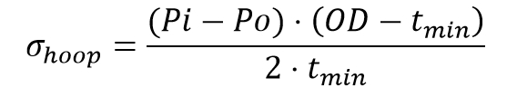
Stress in the pipe wall in the hoop direction is defined by the following basic equation:

Where:
t is the pipeline wall thickness (m);
D is the pipeline diameter (m);
Pi is the internal pressure;
Po is the external pressure.
This equation assumes:
That the hoop stress is the only stress acting;
Giving constant stresses through the pipe wall; i.e. radial stresses by internal and external pressures are negligible.
Whilst all codes use this equation as a basis, the definitions of diameter and wall thickness vary as discussed below, as do the inherent safety factors applied to the usage of the material strength.
Allowable Stress Design Code Pressure
Many design codes reference outer diameter (OD) rather than mean diameter or inside diameter (ID). They also specify the selection of minimum or nominal wall thickness and the prescribed hoop stress utilisation factor. Considered together, these factors combine to influence the overall factor of safety on burst strength of the pipe. Examples of the differences between codes are illustrated below.

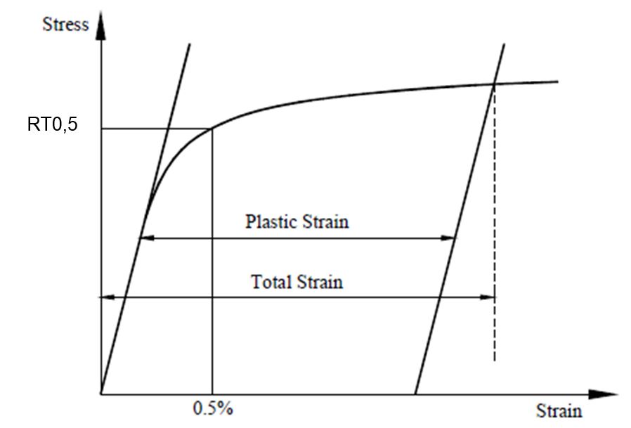
Yield Stress
The yield stress is defined as the stress at which the total strain is 0.5%.
Load Resistance Factor Design Codes
The bursting criteria defined in the LRFD codes such as [13] are also based on thin wall theory. In [13], the basic limit state for bursting is defined as:

This defines the bursting criterion, where:
pli is the local incidental pressure;
pe is the local external pressure;
pb(t1) is the pressure containment resistance based on minimum wall thickness t1 (i.e. after subtraction of manufacturing tolerance and corrosion allowance);
γSC is the safety class resistance factor;
γm is the material factor.
The local incidental pressure is defined as follows, where the ratio between incidental and design pressures (γinc) is normally taken as 1.1:
![]()
And the local external pressure is defined as:
![]()
The pressure containment resistance is defined by:
![]()
Where yielding limit state is given by: 
And bursting limit state is given by: 
Where:
![]()
![]()
fy,temp and fu,temp are the strength derating values for elevated temperatures;
αU is the material strength factor, which is normally taken as 0.96. If supplementary requirement U has been specified a factor of 1.0 may be applied;
αA is the anisotropy factor, which is 0.95 for the axial direction (due to relaxed testing requirements in linepipe specification) and is 1.0 for all other directions.
The above equations are specific to [11], and one should be aware that if using another code such as [6], other equations and methodology would apply.
Other Factors
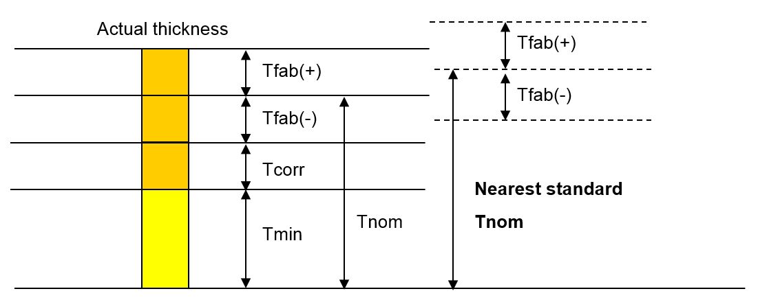
It has already been hinted in the discussions above that other factors contribute to the definition of the nominal wall thickness requirement. The rational for wall thickness specification is normally:
t = tmin + tcorr + tfab(-).
tmin is the minimum wall thickness required for pressure containment;
tcorr is the corrosion allowance;
tfab(-) is the manufacturing under-tolerance on wall thickness.
Having determined the required wall thickness it may be appropriate to round up to nearest standard wall thickness size. These requirements/definitions are illustrated in Figure below.
External Pressure
Hydrostatic Collapse
External overpressure due to hydrostatic head can lead to collapse of the pipe. Collapse depends on ovality, caused by fabrication tolerances, subsequent handling, and, in the case of reeling, the bending of the pipe onto the reel. External collapse of thin walled pipes is primarily driven by the elastic properties of the steel. Ovalisation of the pipe results in the hydrostatic forces on the flat sides being much larger than the hydrostatic forces on the ends. This creates moments within the pipe wall that tend to increase the ovalisation. When elastic and plastic resistance to this ovalisation is overcome, a flattening of the pipe occurs.
The following criterion is taken from [11]. The characteristic resistance is given by solving this equation.

Where:
pel is the elastic collapse pressure for a perfect tube given by:

With t2 = t - tcorr;
E is Young’s Modulus of the pipe material (N/m²);
t is the pipeline wall thickness (m);
tcorr is the corrosion allowance (m);
D is the pipeline diameter (m);
ν is the Poisson’s ratio of the pipe material;
pel is the elastic collapse pressure for a perfect tube (N/m²).
And:
pp is the plastic collapse pressure for a perfect tube given by:

And ovality is given by:

The fabrication factor αfab depends on the linepipe manufacturing process and allows for the effects of cold working, giving a variation between tensile and compressive strength.
Investigations have shown that different external collapse formulae can give significantly different results in deep water, heavy walled applications. It is recommended that the methods defined in [33] or [6] are used as these have been specified with deepwater applications in mind.
Propagating Buckle
The external pressure required to cause a buckle to propagate is lower than is required to collapse the pipe. If the pipe is designed to resist buckle propagation, any local buckle accidentally introduced will not propagate. This is normally the case for pipelines installed in shallow water, where wall thickness is governed by internal pressure containment. As water depths increase, buckle propagation design begins to dominate.
It is possible to design pipelines to exceed the buckle propagation pressure and design instead to the external collapse pressure with adequate mitigation measures. These include the use of buckle arrestors to limit the damage caused if a buckle is initiated.
Since buckles are normally caused during installation and the worst conditions for buckle propagation also occur during installation when the pipeline is empty, this forms the principal design case.
It is normal to use 100% of any corrosion allowance in the analysis.
The critical pressure for buckle propagation, is:

The critical pressure for buckle propagation, as defined by [13] is:

[13] is more likely to be used for such check.
![[Note]](note.png)
Note
In reeling applications, the requirement for buckle arrestors would be problematic due to the resultant strain concentrations in the pipe adjacent to the arrestor during the reeling-on process. A clamp-on external buckle arrestor can be alternatively attached around the pipe after the straightener or straightening process.
Combined Check
Combinations of loads (pressure, axial tension or compression, bending) can lead to yielding or buckling. ASD codes include checks on equivalent stress under combined loads. The LRFD codes, and indeed ASD codes, include criteria for local buckling.
Equivalent Stress
ASD codes specify combined stress criteria. Using suitable yield criteria for combined stress, normally Von Mises, allowable combined equivalent stress is set close to yield. Equivalent stress in pipelines is defined by Von Mises criteria as follows:

In the above equation:
σeq is equivalent stress;
σh is hoop stress;
σl is longitudinal stress;
τ is torsional or shear stress.
Limits for equivalent stress are defined in Table below
Local Buckling
The most common cause of local buckling is excessive bending at the sag bend during pipelay. Normally, a buckle detector is towed along by the laybarge inside the pipeline, enabling the barge to back up and repair buckles on detection.
The localised buckling of the pipe is analogous to the folding of a drinking straw. As the pipe bends, it places the extreme fibres in tension and compression. To partially relieve these stresses, the pipe deflects, ovalising to flatten the areas under stress. The ovalisation reduces the bending stiffness of the pipe. Eventually a runaway point is reached and the pipe buckles, forming “pinch points” that may tear or fracture, with the potential for loss of contents, or in the case of installation, flooding of the pipe. Any axial compression in the pipe adds to the tendency to form a buckle.
Buckle criteria are defined in both allowable stress design codes and limit state design curves ([13] and [6]1). An example of the [6]1 criteria is further illustrated for the wall thickness selection based on reeling criteria.
Reeling
The reeling process introduces strength requirements that are not necessary for S-lay or J-lay processes, [82]. This is because the pipe is plastically deformed during the reeling process. Typically nominal strain in the longitudinal direction is above 1% during single bending cycles and should stay below 5% (this range is covered by the codes). The particular considerations for reeling are:
Buckling due to high bending;
Ovalisation of the pipe;
Cumulative strain due to the yielding process.
Pipelines installed by reel-lay require thicker wall than pipes installed by S-lay or J-lay because of increased ovality for reeled pipes. Indeed, the bending process during reeling-on induces an ovalisation of the pipe. On straightening during pipelay a significant proportion of that ovalisation is recovered but a resultant ovalisation remains in the pipe after installation. Increased ovality reduces resistance to hydrostatic collapse and, for deepwater installations; this ovalisation of the pipe due to reeling may become significant.
For deep water pipelines, installation load during reeling and collapse due to hydrostatic pressure are the main governing factors in determining the pipe wall thickness. If the pipe ovality is over estimated this will lead to a much higher recommended value of the pipe wall thickness.
Therefore, accurate prediction of pipe’s ovality when on the reel and residual, or as installed, ovality of reeled pipes is crucial in determining a lower and yet safe wall thickness to withstand the buckling load due to bending during installation (reeling operation) and collapse pressure when reaching the seabed.
Buckling Due to Bending- API 1111
As explained previously, the pipeline design codes specify the criteria for buckling due to high bending. The buckling formulae specified in [6]1 provide a sound basis for buckling prediction. Generally, it is recommended that buckling criteria to both [6]1 and the local design code be checked and the requirements of the most onerous adopted. Buckling criteria to [6]1 are as follows:

For reeling-on, internal and external pressures (Pi and Po) are zero and therefore this simplifies to:

Where:
![]()

is the ovality
![]()
is the buckling strain under pure bending
Dmax is the maximum diameter at any given cross section;
Dmin is the minimum diameter at any given cross section;
D is the nominal diameter;
t is the nominal wall thickness;
![]() is the design strain;
is the design strain;
f1 is the safety appropriate for the variations in bending strain during reeling;
ε1 is the maximum strain during reeling.
On the reel, the bending is deflection limited. However, during the reeling-on process the pipe just off the reel is not deflection limited yet and is subject to the maximum bending moment. It is in this location therefore that local buckling of the pipe tends to occur during the reeling process, specifically at the welds where strain concentrations will be accounted for due to:
uneven deformation caused by variations in actual material yield stress and strain hardenability between pipe joints and in the weld metal due to scatter in material properties;
variations in cross sectional area (actual diameter or wall thickness) between pipe joints;
stiffening effects of coating and variations in coating thickness;
reduction of yield stress in field joints due to high temperature imposed by field joint coating application during installation; and
undermatch / overmatch of actual weld metal yield stress, relative to actual pipe material yield stress.
Cumulative Strain- [13]
Cumulative strain may degrade the fracture resistance of material, and of particular concern is the fracture resistance of the girth weld area. [13] defines the following requirements for cumulative plastic strain.
Table 2.3 - Cumulative plastic strain criteria
Cumulative plastic strain | Requirement |
≤ 0.3% | No additional requirements |
0.3% to 2.0% | Engineering Criticality Assessment (ECA) – determine material fracture toughness required to tolerate largest weld flaws |
> 2.0% | Additional material tests to determine characteristic strain resistance (DNV supplementary requirement P) |
The Engineering Criticality Assessment requires that a fracture assessment be performed to BS7910 level 3. This assessment would typically be based on the largest weld defects allowed by welding specification and would require additional tests to be performed to quantify the CTOD or fracture toughness of the material.
Further details are provided in the guideline [20] which gives guidance regarding testing and analyses for fracture control of pipeline girth welds during installation by methods introducing cyclic plastic deformation, e.g. installation by the reeling method.
Wall Thickness Selection- Straightener Capacity
During reel-lay installation the pipe is subjected to a reverse curvature in the straightener prior to deployment subsea. Due to the thick nature of deep water reeled pipelines, it is necessary to consider if it is possible to straighten the pipe during installation. A comparison should be made between the maximum plastic moment capacity of the straightener and the plastic moment of the pipe.
The calculation should also take into account variations in the values for yield stress and variations in wall thickness tolerances. The yield strength should include strain hardening from the reeling process and a maximum of SMYS (typically +100N/mm²) should be considered. The wall thickness positive tolerance should also be included (typically +12.5% for [13]).
Post-Reeled Residual Ovality in Pipe
Collapse due to external pressure may determine the wall thickness for deepwater pipelines. Collapse depends on pipe ovality. The residual, or as laid, ovality of a reeled pipeline is required for design calculations to check against pipe collapse due to external pressure and bending.
Collapse Due to External Pressure
The limiting water depth of the pipeline should be calculated based on the criteria of the local code if specified in the respective contract. As API RP 1111 [6] clause 4.3.2.1 does not include an ovality term, which is obviously important for external collapse capacity, an assessment to [13], Section 5, Clause D503 and D504 should be made.
Bauschinger effect
According to [20], the shape of the stress-strain curve will change due to the cyclic plastic straining (the Bauschinger effect, see Section 8.4.2, “Mechanics of Reeled Pipe”). The change in stress-strain curve due to the Bauschinger effect is normally a decrease of the yield strength (typically 15-20 %) but the tensile strength is essentially unaffected. However, in case both the yield strength and the tensile strength are lowered due to the Bauschinger effect it may be necessary to consider this in the assessment, e.g. external collapse capacity.
2.3.4 On-bottom Stability Check
The embedment and the stability of the pipeline depends on the soil characteristics, on the current loads (and wave loads when considering shallower conditions or area with internal waves), on the overall outside diameter and on the weight of the pipe. Checking the horizontal and vertical stability of the pipe aims to eventually adapt its diameter and weight, for example by adding a concrete layer if necessary.
This section gives an overview of the design methodologies.
There are two main guidelines for stability design, namely:
DNV have recently produced a document detailing several aspects of pipelines on-bottom stability:
Load combinations
Weight calculations
Resistance calculations
Design criterion
The guidelines are outlines in the following [21] which is currently available (draft status).
Stability Remedial Measures
The normal approach to stability design is to first increase the submerged weight of the pipe by an optimum combination of thicker wall pipe and concrete weight coating (not compatible with reel lay method). If this is insufficient or not cost effective the alternative approach is to trench the pipeline. Stability on the seabed still needs to be achieved for the installation phase, prior to trenching.
Trenching can be performed in most soil conditions, by ploughing, jetting or cutting. The effectiveness of these trenching methods differs mainly as a result of specific soil conditions and seabed features such as pockmarks, sand-waves and seabed gradients. A full trenching risk assessment should be carried out to identify the most appropriate trenching tool, its performance and associated risks.
The trench can be backfilled to further enhance pipeline on-bottom stability and protection as well as providing natural thermal insulation to heat loss thereby allowing optimisation of coating thickness.
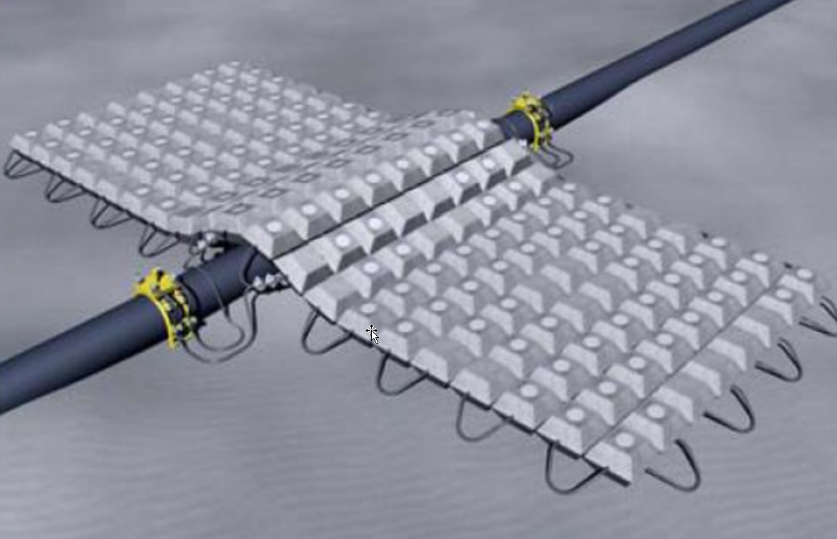
Where trenching can not be employed the following alternatives may be considered.
Rock dump;
Mattresses/saddles/tunnel;
Fronds.
It should be mentioned that mattresses/saddles and fronds only apply to localised sections of the pipeline. It is also worth mentioning that the above remedial solutions are normally much more time consuming and expensive than trenching.
Rock Dump
If large sections of a line need to be stabilised then (in the absence of trenching as an option) rock-dumping would normally be preferred. The material, i.e. rock is low-cost but there are high mobilisation costs for the rock-dump vessel. Post-dump survey of rock-dumped sections is normally required, again increasing costs. In addition, a suitable source of rock is required with access to a marine base at which it could be loaded. It is for this reason that the rock dumping is widely used in the North Sea but rarely in the Gulf of Mexico.
Checks need to be carried out on the possible damage to the pipeline during the rock-dumping operation and if large diameter rock is required for stability then a smaller diameter rock may need to be dumped as an buffer layer to protect the pipeline.
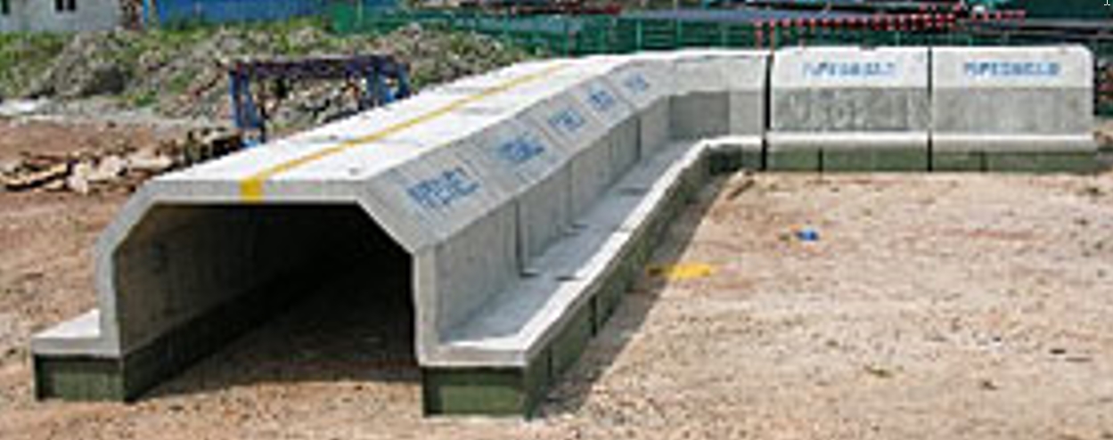
Mattresses/Saddles/Tunnels
Both mattresses and saddles may be used to increase the download, and hence axial and lateral resistance, between the pipe and seabed.
|
|
Concrete Matress | Tunnel |
Mattresses are made up of concrete blocks strung together on polypropylene rope. Depending on the configuration of the concrete segments, they may flex in either 1 or 2 planes and can be made in a large range of sizes.
Mattresses can be sized/weighted to suit a specific application. The addition of iron ore to the concrete gives the ability to increase the weight of the mattress.
Concrete mattresses are widely used to add stability and/or protection to pipelines. Their advantages are that they are:
Cheap;
Simple;
Readily available - they can be taken out on a DSV and used if needed.
The disadvantages are:
They may be removed by trawlers;
They may not be stable in severe sea-states - the edges may lift and the mattress be removed from the pipeline;
They are not attached to the pipeline, which may move from under the mattress.
Saddles/Tunnels are generally made of concrete and straddle the pipeline and can vary in size to suit a specific application. The weight can be reduced by the use of soil anchors to provide additional download and lateral restraint. These will be spaced along the pipeline to maintain stability and are particularly effective in resisting high lateral environmental loads.
Installation is normally carried out using bespoke frames to allow placement without damaging the pipeline; installation can therefore be slow. Saddles/Tunnels can be expensive but in areas of high environmental loading it may be the only option available.
Fronds
In areas of sediment transportation, the use of fronds can be effective in stabilising pipelines or other structures. Fronds, or artificial seaweed, have been widely used for seabed stabilisation and scour prevention in the southern North Sea.
Fronds can be installed on their owns or can be included in concrete mattresses. They work by locally slowing near seabed currents thereby encouraging the deposition of sediment and the formation of a berm of seabed material. Typical frond heights will be of the order of one metre.
The berm will build up rapidly where there is sediment transport and a metre high berm could be built up in about one month for a typical sandy seabed. For silty seabeds, the berm takes longer to establish, perhaps three to four months. Once formed the berm is compact (due to the agitation of the fronds) and durable.
2.3.5 Thermal Design
General
This section considers the basic principles of thermal design. When we refer to thermal design, we are concerned primarily with maintaining temperature within the pipeline product. There are several reasons why this can be important to pipeline operations.
The main concerns are wax formation in oil lines and hydrate formation in gas or multiphase lines.
Wax formation and deposition can be a problem for crude oils containing large chain paraffins (carbon number greater than 30). These crudes are referred to as waxy crudes. The wax is dissolved at higher temperatures and crystallisation occurs as the fluid temperature drops. The temperature at which the wax crystals first form is referred to as the cloud point. At lower temperatures a wax matrix is formed which causes the crude to effectively solidify. The temperature at which this occurs is called the pour point. In operation, the wax will deposit on the ‘cooler’ pipe walls and restrict the flow. Waxy crudes also demonstrate non-Newtonian viscosity behaviour.
Hydrates may form in gas pipelines when water is present. Hydrates are compounds of methane and water that look very much like water ice. The methane molecules are trapped within a cage of water molecules. Hydrates form under conditions of low temperature and high pressure. Therefore production flowlines, where the line pressures tend to be very high, are particularly susceptible.
With both wax and hydrates, a method of prevention is to maintain product temperatures above a minimum formation temperature. This is where thermal design is considered. The two main conditions that the thermal design needs to consider are the steady state operating condition and the transient or shut-down condition. The product temperature will fall as it flows along the pipeline due to conduction of heat through the pipe to the surroundings. The temperature profile of the pipeline can be calculated for the steady-state flow conditions, and so the arrival temperature of the contents at the far end of the line may be determined. If the steady flow condition is interrupted, for example to do maintenance work, then the contents will cool down. The temperature of the contents as a function of time must be determined, with the aim of keeping the temperature at an acceptable level.
Thermal Design of Insulation Systems
Steady State Heat Transfer
For most thermal analyses of pipelines, axial conduction of heat along the pipeline can be ignored and therefore the analysis becomes one of simple radial heat flow. The steady state heat transfer through a layer in a cylindrical system is given, per unit length by:
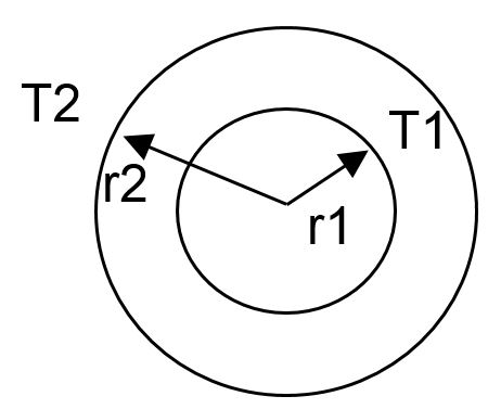

Where
Qr is the heat flow through the layer per unit length;
k is the thermal conductivity of the material;
r1 and r2 are the inner and outer radii of the layer being considered;
T1 and T2 are the temperatures at the inner and outer boundaries of the layer being considered.
The heat flow through the layer can be conveniently expressed in terms of a thermal resistance coefficient, R, as shown below.
 Where
Where 
The heat transfer coefficient, 1/R, defines the thermal performance of the layer in terms of heat transfer per unit length of pipe per unit temperature difference across the layer.
Pipeline Coating Systems
Pipelines are often multi-layer systems, which include the steel pipe wall, anti-corrosion coatings, insulation coating layers and concrete weight coating. With multi-layer systems, an overall thermal resistance coefficient needs to be calculated by summing the contributions of the individual layers as follows:

The overall thermal performance requirement is often defined or specified in terms of an Overall Heat Transfer Coefficient (OHTC), also referred to as U-value, which defines the thermal performance in terms of heat transfer per unit area per unit temperature difference across the total system. This is defined by:

It must be noted that the U-value requires a reference diameter, Dref, because the system area changes through the system thickness. It is normal for OHTC to be referenced to either inside or outside diameter of the steel line-pipe. The unit of U is W/m²K.
Buried Pipeline
When buried, the soil around a pipeline will provide thermal insulation. The effective thermal resistance coefficient for soil, based on the cylindrical system, is:

Where burial depth, b, is as defined in the diagram. This equation is valid only for full burial of the pipe, i.e. b >> D/2.
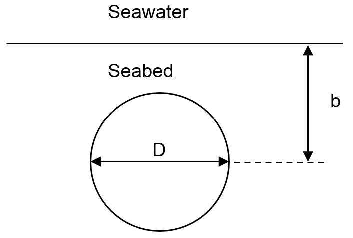
When a pipeline is buried, the thermal resistance coefficient for the soil is included with the other system components in the calculation of OHTC.
Whilst seabed soil can be a good insulator, porous burial media, such as rock dump, may give little in the way of additional insulation if water can flow through the spaces between the rocks and transfer heat to the surroundings.
Steady State Flowing Conditions
Process requirements may define a minimum system temperature under steady-state flowing conditions. This requirement would normally be defined as a minimum arrival temperature for the product. The temperature of the product in the pipeline under steady-state flowing conditions can be determined at any location in the system using the following equation:

Where:
T(x) is the contents temperature at distance x along the pipeline;
Tamb is the ambient seawater temperature;
Tin is the flowing inlet temperature;
OHTC is the overall heat transfer coefficient as defined above;
A is the reference area given byπ Dref;
flowmass is the contents mass flow rate;
Cpcont is the contents specific heat capacity.
This assumes steady state flow conditions, constant fluid properties, uniform insulation and uniform ambient temperature along the pipeline section. It must be mentioned that the above equation applies to a pipeline resting on a relatively flat seabed where the only heat loss is due to surrounding medium. When there is a differential of water depth along the pipeline (i.e. pipeline/riser) or drop of water depth, fluid energy loss and Joule Thomson effects may have a great impact on the temperature loss.
Pipeline Cool-Down
A thermal analysis of the cool-down determines the contents temperature as a function of time, following the shut-in of the line. Cool-down analysis is carried-out for one of the following requirements:
To find the final temperature of the contents after a defined shut-in duration (typically 4 to 20 hours);
To find the time taken for the contents to reach the temperature when wax or hydrates may start to form;
To find the OHTC required to meet a given minimum contents temperature following a given shut-in duration.
Cooldown analysis is normally performed at the outlet from the pipeline, as this gives the coolest contents from the thermal profile analysis.
For transient conduction problems, the rate of change of temperature depends not only on the thermal conductivity of the material (k), but its density (ρ) and specific heat capacity (Cp). At the time of shut-in, heat energy is contained within the contents, the steel linepipe and the coatings, with the amount of energy being a function of the density and specific energy of the layer or component material and the operating temperature of that component or layer. The rate at which that energy leaves the system depends on the thermal resistance or insulation.
A simple approximate method for assessment of cool-down is shown below.

Where:
T(t) is the contents temperature after time t;
Tamb is the ambient seawater temperature;
Tinitial is the contents initial temperature;
OHTC is the overall heat transfer coefficient as defined above;
A is the reference area given by π Dref;
massi is the mass (per unit length) of the pipe contents and steel;
Cpi is the specific heat capacity of the pipe contents and steel.
This equation defines temperature at a point in a shut-in pipeline versus time. This assumes constant fluid properties, uniform initial system temperature, constant ambient temperature and also that the contents and steel pipe are the only layers that contribute to the thermal inertia (i.e. thin coatings), while other layers contribute to the insulation. This assumption is reasonable for pipe with foam coating systems where the contained thermal energy within the coating is low, but becomes conservative for high density coatings such as syntactic PU, where considerable energy may be stored within the coating.
The accurate assessment of cool-down is difficult to perform by hand, and whilst Mathcad or Excel spreadsheets can be set-up utilising finite-difference time-step methods, it is often simplest to use uni-axial finite element analysis.
Other Design Issues
There are a number of additional issues, relating to the coating design, to consider in the thermal analysis. These are not addressed in detail here, but should be considered by the design.
Compression and creep – Polymeric coatings may be subject to elastic compression and creep resulting from the hydrostatic load. In foam coatings compression and particularly creep can be significant and water depth limitations result. Coating compression reduces the thermal performance of the coating by reducing the overall coating thickness and increasing the thermal conductivity of the material due to densification. Glass syntactic and solid pipeline coatings generally demonstrate insignificant compression or creep due to the effective geometric constraint resulting from a continuous coating and the high Poisson’s ratio.
Water absorption – All polymers absorb water over time. This will increase thermal conductivity of the material.
Field joints – Field joints are often of a different material or system to the main pipe coating. The overall performance of the coating and field joints must be considered.
2.3.6 Pipe Expansion Calculations
All of the pipeline design codes specify the requirement to consider expansion and resultant loads in the design of the pipeline and its associated components. They do not, however, specify how the expansion should be quantified. This section defines the principles for determining the magnitude of pipeline expansion, and describes the methods by which it is typically accommodated.
End Expansion
End expansion is due to the pipeline operating loads, namely pressure and temperature and is resisted by friction between the pipeline and its surroundings. If the effects of friction were to be ignored, i.e. assume the pipe was resting on a frictionless surface, the resultant strain due to a change in temperature and pressure can be defined as follows.
Thermal strain is given by:
![]()
Where:
α is the thermal expansion coefficient;
ΔT is the temperature difference relative to the installation temperature.
Strain due to pressure results for two component effects, the end cap force which will expand the pipe and the Poisson’s effect which will contract the pipe. The resultant strain (assuming thin wall theory, D>>t) is given by:

Where:
ΔP is the internal pressure difference relative to the installation pressure (as-laid);
D is the diameter;
t is the wall thickness;
E is the elastic modulus of the linepipe;
ν is the Poisson’s ratio.
The total strain therefore is the combination of pressure and temperature effects given by:

In reality this idealised condition does not occur and restraint to expansion is provided by the seabed friction and any externally applied restraints. The seabed friction builds cumulatively from the pipeline end back along the pipeline to a point at which it is able to fully react to the expansion forces. At this point the pipeline is fully constrained and no expansion occurs beyond this point. This point is referred to as the virtual anchor. This is illustrated in Figure below.
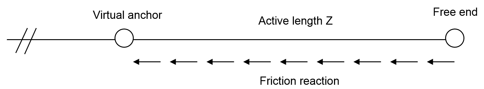
The strain will vary from the ‘frictionless’ strain presented in the equations above at the free end down to zero at the virtual anchor point. This strain does not necessarily vary linearly.
If one considers a thin element of pipe, of length δx, within the active length, a distance x from the end, the expansion of that element, δu, is given by:
![]()
Where ϵx is the strain at distance x from the end.
One can therefore determine the total end expansion, U, by integrating this equation over the active length z, giving:

Anchor Load and Active Length
The virtual anchor occurs at the point where the cumulative friction restraint balances the expansion forces within the pipeline. The anchor force required to restrain the pipeline is given by:

At the pipeline end it may be non-conservative to include residual lay tension in the anchor load as the tension close to the pipe end will be locally relieved to some extent by contraction of the pipe following laydown.
Assuming constant friction, the cumulative frictional restraint at location z is given by:
![]()
Where:
![]() is the frictional force per unit length.
is the frictional force per unit length.
For a pipeline resting on the seabed, the frictional force can be specified using simple Coulomb friction;
![]()
Where:
μaxial is the Coulomb friction coefficient;
Ws is the submerged weight of the pipeline per unit length.
When the pipeline is buried the friction force per unit length depends on the soil conditions, but for example is estimated using equations similar to:
![]()
Where:

γs is the submerged weight of soil;
ka is the active lateral pressure coefficient;
H is the depth of cover over top of pipe;
Do is the outer diameter of the pipe over coatings.
One can equate Ffriction to Fanchor to determine the active length z.
One can define the temperature at a location x from the pipeline end as:
![]()
Where:
x is the distance along the pipeline;
ΔT is the temperature differential at the pipeline end;
λ is the decay length over which the temperature differential drops to 1/e of its initial value given by:

Where:
htotal is the total heat transfer coefficient;
![]() is the mass flow rate;
is the mass flow rate;
Cp is the fluid specific heat capacity.
Assuming constant friction and pressure, the active length is given by:

The end expansion is given by:

Pipeline Walking
When a pipeline is laid on the seabed and heated, it will tend to expand. The expansion is only resisted by the friction generated by the seabed. When the pipeline is cooled, it contracts but the effects of seabed friction mean that the pipeline ends cannot contract to the original position. On subsequent heat-up and shutdown cycles, the pipeline ends cycle between the fully heated position and the cool-down position; this behaviour is addressed in the traditional approach to pipeline expansion design.
However, in some cases thermal cycling is accompanied by global axial movement of the pipeline, this global movement is termed pipeline walking. Over a number of start-up and shutdown cycles pipeline walking can lead to significant global displacement of the pipeline, which can overstress expansion spools or jumpers.
Walking is a phenomenon that occurs in short, high temperature pipelines. The term ‘short’ relates to pipelines that do not reach full constraint in the middle, but instead expand about a virtual anchor point located at the middle of the pipeline. With the current increase in pipeline operating temperature, ‘short’ pipelines can be many kilometres in length.
The mechanism behind pipeline walking under thermal transient loading is outlined in the following section.
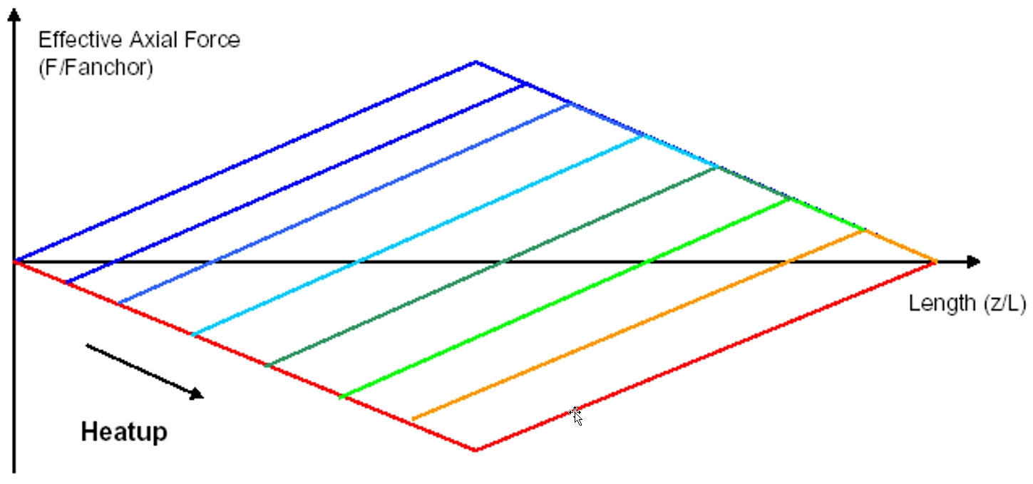
The basic pipeline walking mechanism can be understood by interpreting the shape of the operating (compressive) and shutdown (tensile) force profiles of a pipeline. In the general transient case, the changes in force profiles through the transient heat-up cycle and the local displacements that occur along the line are also of fundamental importance. A typical force profile envelope is illustrated in Figure below Figure 2.3, “Force Profile Envelope for a Fully Mobilised Pipeline” .
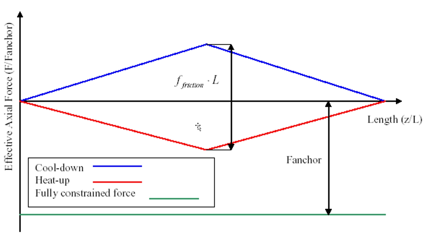
Figure 2.3, “Force Profile Envelope for a Fully Mobilised Pipeline” shows the force profiles for a fully mobilised ‘short’ pipeline, in the fully heated position and the cool-down position. The fully-constrained force generated by pressurising and heating the pipeline, is also shown. For a pipeline to be fully-mobilised the fully constrained force (![]() ) must exceed the height of the force envelope defined by axial friction (
) must exceed the height of the force envelope defined by axial friction (![]() ). This definition of a ‘short’ pipeline is fundamental, as such lines are the most susceptible to pipe walking.
). This definition of a ‘short’ pipeline is fundamental, as such lines are the most susceptible to pipe walking.
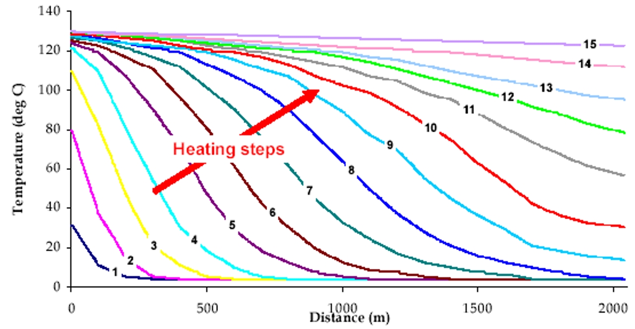
The key to the ‘transient’ walking phenomenon is shape of the thermal profile developed over time as the pipeline heats-up. As hot fluids enter the cold pipeline, heat is lost to the surrounding seawater and the fluid quickly cools to ambient temperature. With time, the pipeline gradually warms until hot fluid is discharged at the far end of the line. A typical set of heat-up thermal transients is presented in Figure Figure 2.4, “Typical_Thermal_Transients”.
The transients cause the pipeline to expand, resulting in a force profile on first load as shown in Figure 2.5, “Example Force Profiles – First Heat-up”. In this and all subsequent plots tension is shown as positive, compression as negative.
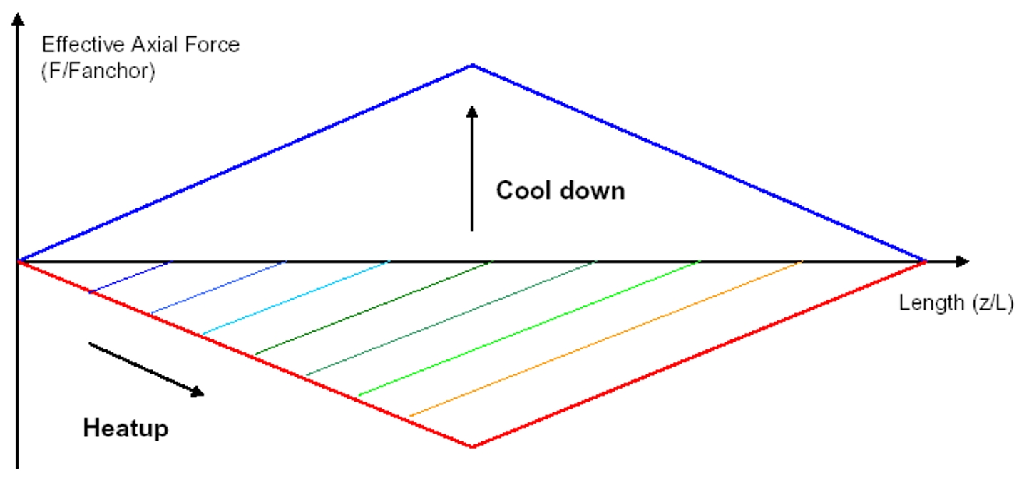
The profile shows the first heating and cool-down cycle for the pipeline from its as installed position. The compressive axial force gradually builds up in the line as the pipeline heats and more pipe is mobilised. When the pipeline becomes fully mobilised a virtual anchor forms at midline and the pipeline expands from this point towards the hot and cold ends. When cooled, the pipeline contracts about the virtual anchor at mid-line. Cooling causes the pipeline to go into effective axial tension (shown as blue).
On the second and subsequent heating cycles, the force in the pipeline builds up in a different manner because of the residual axial tension developed in the pipeline on cool-down. The force profiles as the pipeline heats up on second load are presented in Figure 2.6, “Example Force Profiles – Second Heat-up” .
Pipeline walking occurs over each thermal cycle, and although walking occurs on first cycle, it is the second and subsequent cycles which dominate the process. Therefore, the second load response of the pipeline has to be considered in detail to understand the walking mechanism.
The walking mechanism under thermal transient loading is quite complex and can only be understood by examining the relationship between the thermal transient, the force profile and the displacement of the pipeline at individual time steps during the heat-up process. Suppose at time ‘t’ the pipeline is loaded with the thermal profile shown in Figure 2.7, “Temperature Profile at Time t”.
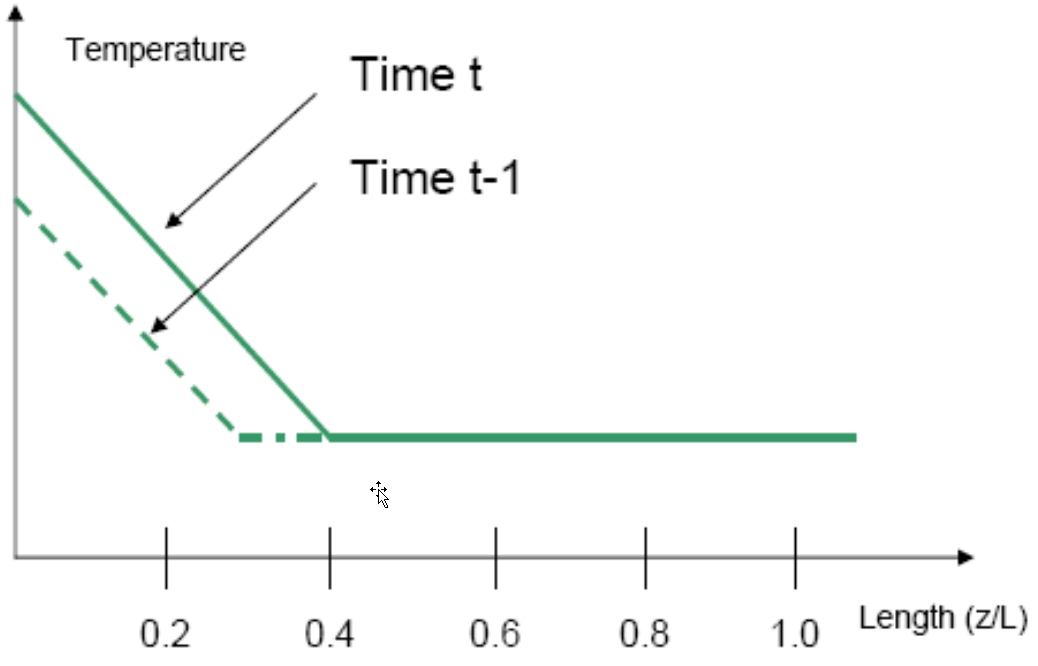
In the temperature profile shown in Figure 2.7, “Temperature Profile at Time t”, the thermal transient is heating the first 40% of the pipeline, downstream of this it remains at ambient temperature. Heating the first part of the pipeline causes the hot end to start expanding; which results in a force profile change, shown in Figure 2.8, “Force Profile at Time t”.
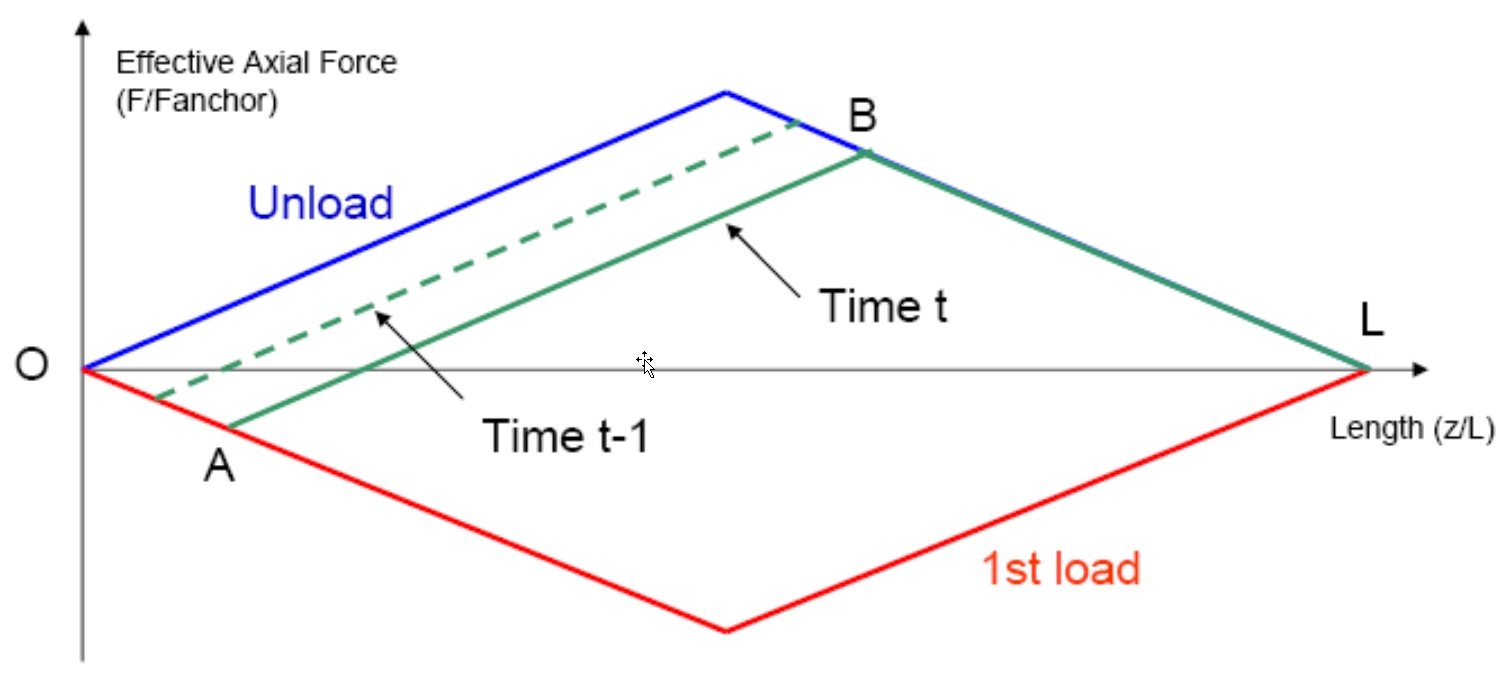
As the pipeline heats up and starts to expand at the hot end, a virtual anchor forms (at A) and expansion occurs towards the hot end between O and A. In order to maintain force equilibrium a second virtual anchor must form (at B) and between the virtual anchors the expansion is towards the cold end. Downstream of virtual anchor B, the pipeline has not been mobilised, therefore there is no change in force along this section of pipe.
The incremental displacement of the pipeline between time ‘t’ and ‘t-1’ is presented in Figure Figure 2.9, “Incremental Displacement between Time t and t-1”. In the plot, positive displacement represents movement towards the cold end.
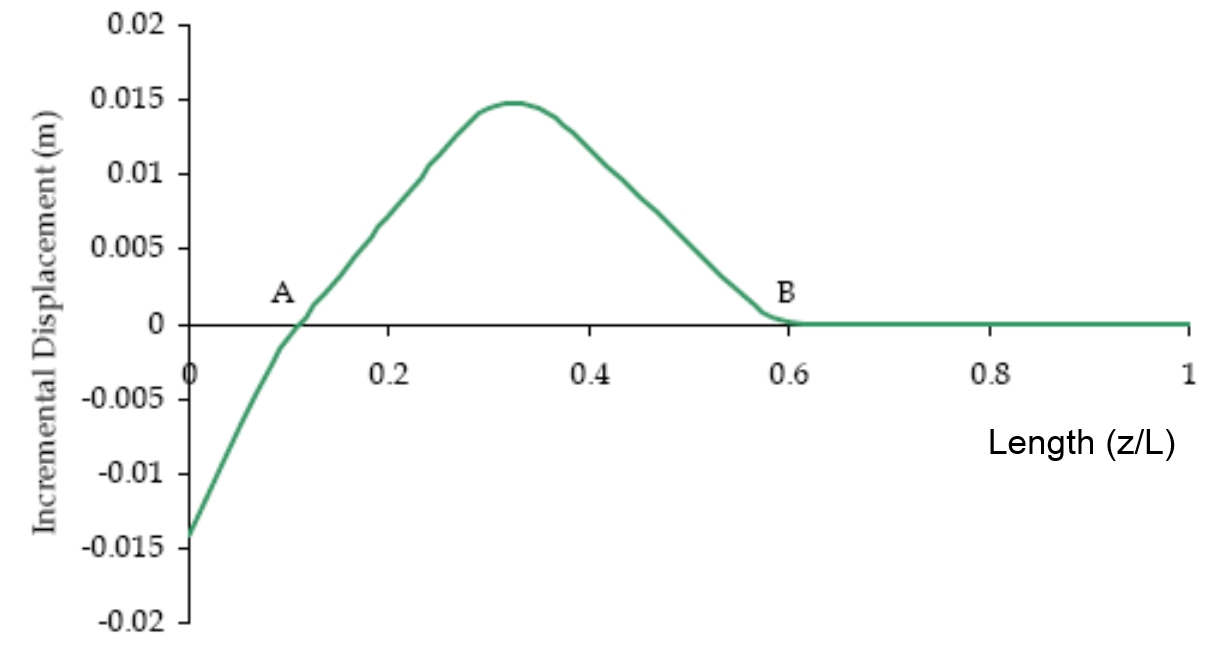
Figure 2.9, “Incremental Displacement between Time t and t-1” clearly shows that during the time between ‘t-1’ and ‘t’ the pipeline is expanding towards the hot end between O and A. The virtual anchors are shown as points with zero displacement. Between the virtual anchors, the pipeline is expanding towards the cold end. This asymmetric displacement along the pipeline is the cause of pipe walking.
As more of the pipeline heats up, the virtual anchors A and B must move to maintain force equilibrium, until the whole pipeline becomes fully mobilised and a single virtual anchor forms at the centre of the pipeline. Figure 2.10, “Force Profile – Position of Virtual Anchors – 2nd Load” shows the force profile for subsequent thermal steps, until full mobilisation of the pipeline at the cold end.

If the incremental displacement over subsequent time increments is considered, it is clear that the asymmetric expansion continues. Figure 2.11, “Incremental Displacements to full mobilisation” shows the incremental displacement until full mobilisation occurs.
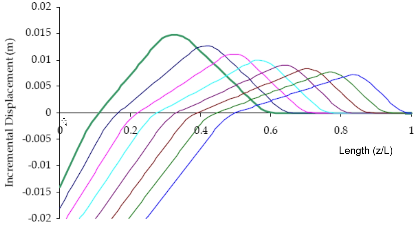
The incremental displacement plot shows the movement of the hot and cold virtual anchors as the pipeline continues to heat up. The hot anchor tends towards the middle of the pipeline, whilst the cold anchor tends to the cold end of the pipeline, leaving a single virtual anchor at mid-line when full mobilisation is reached. Pipeline walking is evident in the plot by the fact that the displacement of the midline is always positive until the anchor forms after which the incremental displacement is zero.
Once full mobilisation has occurred the cold end begins to expand as the temperature continues to rise. However, because of the expansion asymmetry earlier in the heat-up cycle, the middle of the pipeline has already moved towards the cold end. This displacement is the ‘walk’. Once full mobilisation occurs, the midline remains stationary and walking stops. This is an important rule governing pipeline walking.
With each shutdown, the pipeline unloads and contracts about the midline virtual anchor. Because the pipeline cools uniformly along its length, no walking or recovery occurs during cool-down. This leads to a global shift or ‘walk’ along the whole length of the pipeline, towards the cold-end.
When the pipeline is re-heated, the process starts again. The transients cause asymmetric expansion along the length of the pipeline, the whole line moves towards the cold end, full mobilisation occurs and the mid-line becomes an anchor, on cool-down the pipe contracts equally about the midline anchor. With each cycle, the pipeline walks towards the cold end. The displacement of the centre of the pipeline over five heat-up/cool-down cycles is presented in Figure 2.12, “Mid-line displacement for 5 load cycles (typical)”.
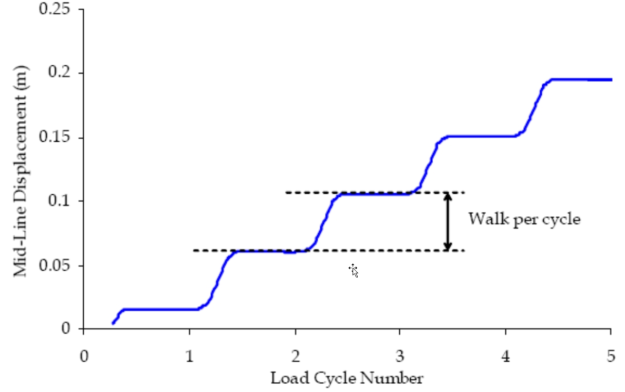
The method of dealing with pipeline walking is included in the design guideline of the recent SAFEBUCK JIP which provides details and analytical equations, ideally suited to conceptual design, to assess the likelihood of walking occurring and to calculate the upper bound walk per cycle (Reference is also made to OTC 17945 – 2006).
Spool-piece Design
In offshore applications, it is normal to minimise the transmission of pipeline expansion loads through to structures by the use of spool-pieces or flexible jumpers.
Typical practice in the North Sea and shallow developments around the world is to use a doglegged rigid spool. The spool length is sized to be sufficient such that the end expansion can be accommodated by bending of the spool, without either the spool being over-stressed or the riser, piping or structure to which it is attached being over-stressed.
In deep-water applications, flexible jumpers can be used to connect the pipeline to the structure. These have been extensively used in Brazil and West of Shetland. Manufacturing capabilities limit the maximum diameter for which flexible pipes are available and so generally they are limited to flow-line diameters.
|
|
Shallow Water Spool | Deepwater Spool |
However, for the majority of deepwater projects rigid spools are used. In the Gulf of Mexico and West of Africa, vertical connection spools are the current “unofficial” industry standard. Such connection systems often present difficulties for the pipeline engineer since they are very sensitive to both expansion of the pipeline and differential settlement between this point and a more rigid connection such as a wellhead or manifold. Resolving the complex problems in this area requires careful engineering and should be treated as a high risk aspect of the design process.
2.3.7 Global Buckling
The majority of hydrocarbon products offshore are transported through subsea pipelines at higher temperatures and pressures than the ambient surrounding environment. This has the following effects:
The differential temperature and pressure causes the pipeline to expand;
The pipeline’s expansion induces an axial compressive force (or driving force) along the pipeline’s length;
This force can sometimes be large enough to cause the pipeline to buckle on the seabed or within a pipeline trench, in the direction of the least resistance.
| Note All rigid pipelines have the potential to buckle. The forms of buckling that may occur are:
|
Buckling can cause the stresses and strains in a pipeline to exceed the operability limit of the pipeline. This could lead to loss of backfill cover, exposure on the seabed, plastic deformation or in the extreme cases loss of containment.
The problems of upheaval and lateral buckling are very much non-linear in nature and therefore generally require the application of finite element based analysis techniques for the accurate simulation of pipeline response. There are however some simple first pass analytical methods which are briefly described in the following sections.
2.3.7.1 Upheaval Buckling
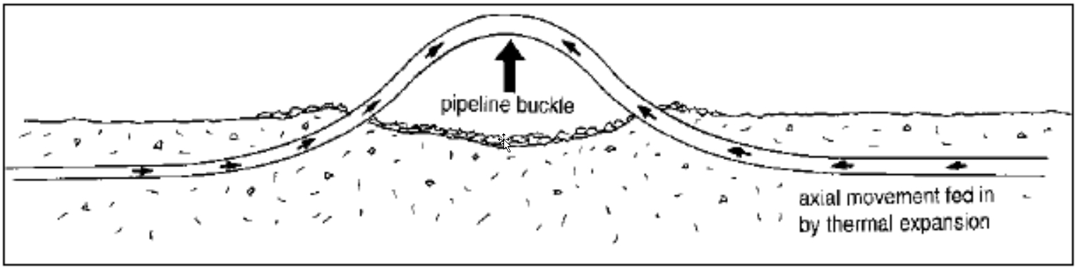
Upheaval buckling (snap buckling) is the gross vertical movement of a pipeline which occurs when the driving force is sufficient to overcome all resistive forces. Snap buckling will occur relatively quickly once the axial force in the pipeline first reaches the critical buckling force. An exaggerated pipeline buckle is shown in Figure 2.13, “Pipeline upheaval buckle” below.
Cyclic ratcheting is a mechanism by which a buried pipeline progressively works its way through backfill material due to driving forces induced by a number of production start-up and shut down cycles. Progressive cyclic ratcheting can therefore lead to the situation where snap buckling is then likely to occur.
In general the occurrence of upheaval buckling is sensitive to the following conditions or combination of conditions that may exist along the pipeline:
|
Axial Compressive Force
As described in Section 2.3.6 the section of pipeline away from the ends become fully restrained by the axial seabed friction. The method for determining the locations at which the pipeline is fully constrained is shown in Section 2.3.6. Care should be taken to select appropriate friction coefficients in this assessment. Where calculating end expansion a lower bound friction value should be use; where calculating virtual anchor locations for upheaval buckling analyses an upper bound friction value should be used.
In the fully constrained section of the pipeline the effective compressive axial force is given by:

Where:
Heff is residual lay tension;
Δpi is internal pressure difference relative to as laid;
Ai is internal cross-sectional area;
ν is Poisson’s ratio;
As cross-sectional area of steel;
α Coefficient of expansion;
ΔT temperature difference relative to as laid.
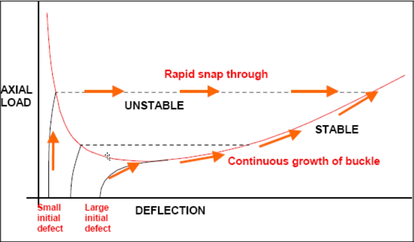
The pipeline will not experience upheaval buckling unless this effective axial compressive force exceeds the buckling force. The magnitude of the buckling force depends on the initial size of the pipeline out-of-straightness as explained below and shown in Figure 2.14, “Prop buckle instability”.
The transverse deflection of the pipeline at the out-of-straightness will initially be progressive as the load increases. However, being a strut buckle it will reach a point of elastic instability and will then exhibit rapid deflection, i.e. ‘snap-through’, until a stable condition is reached again.
The axial restraint of the pipeline is reduced at the buckle and pipe will ‘feed-in’ to the buckle as the pipeline expands.
The ‘snap-through’ response of the pipeline is illustrated in Figure 2.14, “Prop buckle instability”. The deflection/load paths are illustrated for 3 initial deflections. With a small deflection a high axial load can be withstood without significant deflection. If the instability load is reached, however, the snap-through response is substantial. A large deflection will exhibit greater initial deflection but the movement of the pipeline will be stable.
Pipeline Geometry and Route Imperfections
Any vertical or lateral Deviations of a perfectly straight pipeline are defined as Out Of Straightness (OOS) events. OOS events indicate the locations where upheaval buckling or lateral buckling are most likely to occur along a pipeline route.
OOS events can be caused by:
Imperfections such as boulders, sand waves, trawl scars, etc along the pipeline route;
Imperfections in the pipeline trench after burying and trenching operations such as local collapse/slumped material from the trench wall under a pipeline or poor trencher control in variable soil conditions.
Due to the presence of imperfections the force required to buckle over an OOS event will be less than the force needed to buckle a perfectly horizontal pipeline. It is for this reason that OOS events are critical in assessing buckling.
An OOS event is typically described in terms of imperfection height and the pipeline wavelength over which it occurs. During a predictive upheaval buckling (UHB) analysis conservative estimates of the required download resistance have in the past been derived by using natural or theoretical pipeline wavelengths for a given imperfection height. This “prop” wavelength corresponds to the minimum and most onerous wavelength for a pipeline spanning a short imperfection.
Where possible the actual pipeline wavelengths should be used in UHB analysis to give a more realistic estimation of rock dump required. Natural or “prop” type wavelengths should be assessed as the more onerous case, if required, to quantify sensitivity and risk.
Note for the pipeline to follow the seabed, the actual wavelength must be greater than the natural wavelength. It is normal practice to consider a range of imperfection heights, generally from 0.1m to 0.5m, at increments of 0.1m, to provide a measure of the pipeline system sensitivity to UHB.
This also serves as a guide for trenching operations to identify critical areas along the route.
Uplift Resistance
The uplift resistance comes from the combination of the pipeline operating weight and any cover that may be on the pipeline from either natural or mechanical backfill, or some other form of download, normally rock-dump.
The soil uplift resistance component is a complex interaction as this varies with the type of soil, rate of loading and the degree of consolidation. Uplift movements of the pipeline operating conditions should be limited to within the range of elastic soil movements to prevent ratcheting.
This is where a pipeline undergoes repeated shutdowns and restarts at high temperatures causing significant displacements to occur; it is then possible for a gap to form between the crown of the imperfection and the bottom of the pipe that can then be filled in with soil. If the temperature is reduced the pipeline is unable to return to the original position resulting in an increase in the initial imperfection amplitude which in turn reduces the soil cover height and buckling temperature. If there are a number of shutdown/restart cycles the pipeline will gradually move through the cover and/or eventually fail by upheaval buckling as the buckle temperature reduces due to the increasing imperfection amplitude.
For embedment depth, a pipe-soil interaction model gives the following formulae:

Where: qs is the uplift resistance of a cohesionless sand cover (N/m)
g is the submerged weight of the soil (kg/m3)
g is the acceleration due to gravity (m/s2)
H is the height of cover (m)
Do is the outside diameter of the pipeline (m)
f is an empirical uplift coefficient (typically between 0.1 and 0.5)
The total downwards force is hence equal to:

Where: Wsp is submerged weight of the pipeline (kg/m)
Potential Failures Caused by Upheaval Buckling
The principal failure conditions associated with upheaval buckling are:
Local buckling in the overbend;
Increased snag potential from trawl gear hooking;
Loss of any local thermal insulation from soil cover.
Local buckling due to the upheaval itself has a low probability of occurrence and generally upheaval buckling is considered a significant problem only in areas where there is a potential for third parties, typically trawlers, to snag on the pipeline.
Design Methodologies
A number of different approaches are available for the analysis of potential upheaval buckling features. A simple analytical approach developed from the results of the Shell JIP on upheaval buckling is presented below. More accurate methods include the use of general purpose finite element analysis packages such as Abaqus, specialist FE packages such as SAGE Profile and problem specific packages such as PC Upbuck or LR-Star. Other complimentary software products include LR-Condense, which is an interactive graphics program developed specifically to de-spike and smooth raw OOS data for use in an upheaval buckling analysis.
The download required for stability in the operating condition, W, as given by Palmer & al is:

Where:
Seff is the effective axial compressive force;
wo is the installation submerged weight;
δ is the OOS height;
E is the elastic modulus of the linepipe steel;
I is the second moment of area of the pipe section.
Design of Submarine Pipelines Against Upheaval Buckling by Palmer, AC, Ellinas, CP, Richards, DM and Guijt, J. OTC 6335 - 1990
This is a simplified semi-empirical method for calculating the download required using an idealised imperfection defined in terms of amplitude, which has the same amplitude and wavelength as the surveyed imperfection and assumed to adopt the minimum wavelength possible due to the self-weight. This assumed half-wavelength is conservatively calculated from the following equation:

2.3.7.2 Lateral Buckling
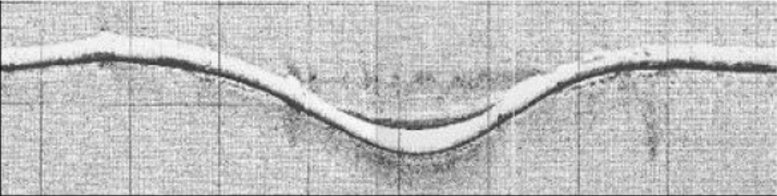
Lateral buckling of the pipeline can occur when the pipeline is laid onto the seabed. As with upheaval buckling it occurs within the constrained section of the pipeline when the axial compressive force overcomes the perpendicular restraint causing the pipeline to move. The perpendicular restraint in this case is provided by lateral friction between the pipe and the seabed. A pipeline lateral buckle is shown in Figure 2.15, “Typical Lateral Buckle from Side-scan Sonar Imag” below.
Unlike upheaval buckling, where movement is restricted to the point where the pipe breaks through the soil restraint and will only occur in the upwards direction, in lateral buckling the restraint is considerably more uniform and the pipe can move in both lateral directions. This generally means that the buckles are able to form in higher mode shapes and over greater lengths, thereby resulting in lower strains than may typically occur in upheavals. However, with the lateral restraint generally being less than the upheaval restraint in a buried pipeline, the propensity to buckling is greater.
Again, the factors of compressive axial force, an initial lateral OOS and insufficient lateral restraint are requirements for lateral buckling to occur. For a pipeline on the seabed, the lateral imperfections will result from undulations in the as-laid routing. As lateral buckling is a problem normally associated with smaller diameter lines, it is possible that trawling interaction can introduce an OOS and initiate a lateral buckle.
Restraint to lateral movement is provided by soil friction. On granular soils, the lateral movement of the pipe will tend to push up a berm of soil thereby increasing the restraint as the buckle progresses.
Design Methodologies
The method of dealing with lateral buckling is included in the design guidelines of the recent SAFEBUCK-JIP and HOTPIPE-JIP.
The HOTPIPE Project is a Joint Industry Research and Development Project, whose overall objective is to prepare a DNVGL Recommended Practice (DNVGL-RP-F110 in preparation) to be used in structural design of high temperature/high pressure pipelines. The design criteria are based on the application of reliability methods to calibrate the partial safety factors in compliance with the safety philosophy established by [13].
The method shown below is for information only and is based on the simplistic method developed by Hobbs. An analytical method has been developed by Hobbs (Hobbs, 1984 and Hobbs and Liang, 1989) which defines the load in a buckled pipeline, the resultant maximum deflection and the corresponding maximum bending moment. The theory is based on force equilibrium and displacement compatibility after a lateral buckle has formed in a theoretically straight pipe. The pipeline is treated as a beam-column under axial load and the linear differential equation of the buckled portion is solved for the deflected shape. Other assumptions and restrictions are that the pipe material remains elastic and that initial imperfections are not considered. The method is also restricted to small rotations.
The method traces the equilibrium path in terms of buckle length and fully restrained axial force.
For a given buckle of length L the compressive effective axial force away from the buckle Po is given by:

Where:
E represents the modulus of elasticity
μA is the coefficient of axial friction
μL is the coefficient of lateral friction
W is the submerged weight of the pipeline
A is the Steel area
E is the Young’s modulus
I is the Second moment of area
L is the Buckle length corresponding to P0
The effective compressive axial force within the buckle, P, is given by:
![]()
And the maximum corresponding buckle amplitude, y, is given by:
![]()
The maximum bending moment, M, is calculated from:
![]()
The coefficients k1 – k5 for the fundamental modes, taken from Hobbs (1984), are given below in Table 2.4, “Coefficients for Lateral Buckling (after Hobbs, 1984)”.
Table 2.4 - Coefficients for Lateral Buckling (after Hobbs, 1984)
Mode | k1 | k2 | k3 | k4 | k5 |
1 | 80.76 | 6.391 x 10⁻⁵ | 0.500 | 2.407 x 10⁻³ | 0.06938 |
2 | 4π2 | 1.743 x 10⁻⁴ | 1.000 | 5.532 x 10⁻³ | 0.1088 |
3 | 34.06 | 1.668 x 10⁻⁴ | 1.294 | 1.032 x 10⁻² | 0.1434 |
4 | 28.20 | 2.144 x 10⁻⁴ | 1.608 | 1.047 x 10⁻² | 0.1483 |
∞ | 4π2 | 4.705 x 10⁻⁵ | 4.705 x 10⁻⁵ | 4.4495 x 10⁻³ | 0.05066 |
Hobbs, R, In-Service Buckling of Heated Pipelines, Journal of Transportation Engineering, vol 110 No.2, March 1984.
Hobbs, R and Liang, F, Thermal Buckling of Pipelines Close to Restraints, International Conference on Offshore Mechanics and Arctic Engineering, The Hague, 1998.
The following factors need to be considered when analyzing pipelines susceptible to lateral buckling:
The above formulation is based on a pipeline having sufficient length to develop full axial constraint away from the buckle length, such that axial feed-in can take place over the slip length. Analytical solutions based on the development of full axial constraint do not adequately model the behaviour of pipelines operating within the expansion zone;
The formulation assumes an idealized straight pipe, and therefore takes no account of any initial imperfection that may be present in the pipeline; and
The theory assumes a single buckle forming in an otherwise straight pipe. In practice, multiple buckles can develop. Feed-in will not be concentrated at one location.
The usual approach to lateral buckling is the use of non-linear finite element analysis using general purpose FEA packages such as ANSYS or ABAQUS (as further illustrated in Figure 2.16, “Lateral Buckling Assessment by FEA”).

2.3.7.3 Mitigation Measures
The aim of the design strategy is to limit the feed-in to any particular buckle. This can be achieved by ensuring a large number of buckles or by limiting the thermal feed-in. The available methods are discussed here.
Buckle Initiation Techniques
Since the formation of the buckle is the key uncertainty it is useful to discuss ways in which buckle initiation can be engineered. There are a number of methods which have been employed or are currently proposed to initiate buckling at a controlled spacing; these include:-
Inherent Imperfections
This is not really an engineered initiation technique; the approach is simply to rely upon the OOS features inherent in a subsea pipeline. Subsea pipeline installation is far from precision engineering. Even the best-controlled DP barge must have some sway and yaw movement transverse to the lay direction. Inevitably, this leads to imperfections in the as-laid pipeline. In addition, there will be vertical OOS associated with the local bathymetry. The evidence from large trunk lines is that these inherent imperfections are large enough to initiate regular buckling.
The main difficulty is to know in advance the magnitude and frequency of the OOS features – clearly this will depend on several factors; pipe stiffness, type of lay vessel, installation sea state, wind, water depth and others. The challenge is therefore developing an approach that will allow the development to proceed with confidence, given this lack of knowledge. A potentially low cost solution related to this approach is to request that the lay contactor deliberately avoids very straight lines, or deliberately introduces regular offsets within the lay corridor.
Snake-Lay
This is the most common approach to lateral buckle initiation used to date. The pipeline is laid in a series of gentle curves as illustrated in Figure 2.17, “Typical Snake Lay Configuration (exaggerated vertical scale)” (there are variations on this theme including a continuously curved lay).
The figure shows the key parameters in the snake lay; pitch, offset and bend radius. The snake pitch is the half-wavelength, defined as the distance between successive snake crowns. The offset is the distance from the lay centre-line to the crown of the snake and the bend radius is the average lay radius around the bend. Under this design philosophy, buckles are supposed to form at the centre of each of these snakes. These are true localised lateral buckles and not benign expansion of the snake crowns; this is illustrated in Figure 2.18, “Buckling Response from Snake Lay”, which shows the results from a FE analysis of a snaked pipeline.
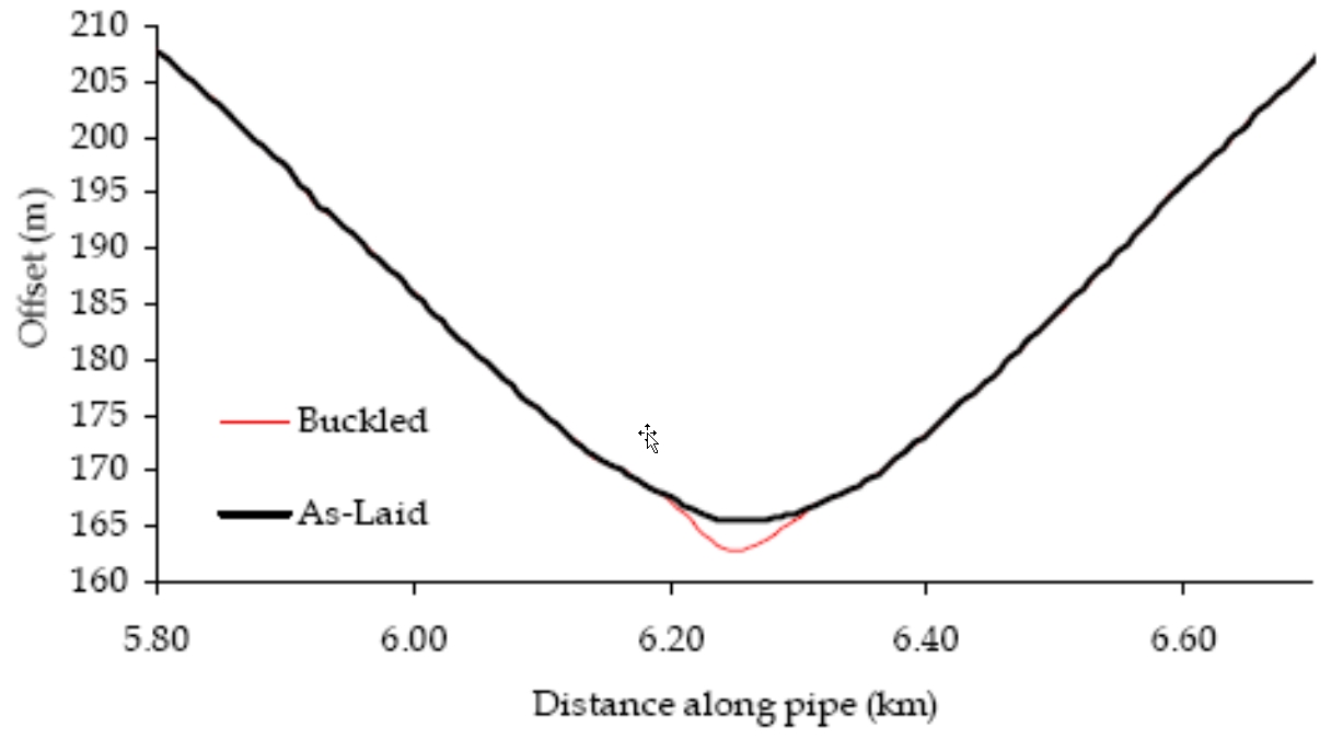
In the idealised situation, a buckle forms at the crown of each snake. However, there are significant problems with the method and uncertainty over whether the method is robust enough to work given practical variations in seabed response. In principle it is possible for the pipeline to “miss” a snake crown, i.e. for it to feed-through a crown without buckling. This can occur for a number of reasons. For example the lateral friction at the snake may be higher than anticipated or a buckle could form between snake crowns, reducing the driving force at the crown below the critical value.
The approach does give the designer some degree of control. The likelihood of buckling can be increased by decreasing the bend radius (although this is ultimately limited by the minimum lay radius capability of the lay vessel). The frequency of buckling can be increased by reducing the snake pitch; although this is limited by the potential for buckles to localise, feed-through and coalesce.
Vertical upset
Pipeline buckling can be initiated in either the horizontal or vertical direction. If the pipeline is laid on an uneven seabed, then an initial vertical movement is highly likely to develop into a lateral buckle. This approach takes advantage of this fact. The technique works by deliberately introducing significant vertical OOS at a number of points along the pipeline. Two techniques have been employed:
Sleepers
Gravel dump
The sleeper technique employs a large diameter pipe joint laid perpendicular to the lay route to provide the out-of-straightness. The sleepers are installed prior to pipe lay at the appropriate spacing. The lay vessel is then required to lay the pipe over the centre of the sleepers. This has the attraction that the friction between the pipe and the sleeper can be minimised by coatings. In addition, the pipe to each side of the sleeper is suspended above the seabed and therefore experiences little frictional restraint. This has the knock-on benefit of reducing the cyclic load in the buckle allowing an increase in the design buckle spacing. In the gravel dump option, the sleeper is replaced by a gravel berm; otherwise the concept is identical.
The approach has the advantage that it reduces the importance (and uncertainty) of the pipe-soil interaction. However, there is still the concern over buckling occurring away from the desired location and it does introduce an additional plane of bending. It can also result in significant pipeline spans; these are susceptible to vortex-induced vibrations and may be a fishing hazard. In addition, the trigger load for upheaval buckling tends to be higher than lateral buckling and the height of the vertical upset may be unrealistically large for very stiff pipes (or PIP systems).
Buoyancy
In this approach discrete lengths (typically 5 or so joints long) of pipe are installed with additional buoyancy on them; these lengths are the intended buckle initiation sites. The buoyancy is chosen so that the operational submerged weight is a small fraction (typically 10%) of the normal pipe submerged weight. A similar approach has been suggested for concrete coated pipelines, whereby sections of lightly coated pipes are installed at regular intervals. This approach could also be combined with the vertical upset solution but could not easily be combined with the snake lay solution due to the difficulty of laying a light pipe around a curve.
The method works in two ways. Firstly, during pipelay, the section of pipe with buoyancy will be positively buoyant. This means that it tends to form vertical imperfections as it is laid down. This is further exaggerated by the increase in outside diameter associated with the buoyancy modules.
These vertical imperfections coupled with the effect of any lateral current loads will tend to produce a natural out-of-straightness at the chosen location. Secondly, because the operational submerged weight is so low, the lateral frictional restraint is reduced. Consequently, the buckle initiation force is also reduced. These combined issues mean that the pipe is more likely to buckle at the locations where the buoyancy is applied.
There is a further advantage; since the lateral friction is reduced, the severity of the bending (for a given design condition) is also reduced. Consequently, the integrity of the pipe within the buckle is improved. The drawback with the approach, as with others, is that it is difficult to guarantee that the pipe will buckle exactly where the designer intends.
Sleepers
Sleeper can be used to initiate buckling of the pipeline at defined locations. It consists in supports laid on seabed on which the pipeline is laid. The supports are generally made in steel, or steel+concrete for shallow water depth, reducing the friction coefficient compared to soil. The pipeline is laid following an S-Lay mode as described here above. Additionally, submerged weight of the curved section can be reduced, by adding buoyancy modules or low-density coating, to ease the lateral displacement of the line. When the pipeline will be submitted to lateral displacement, it will preferentially move at sleepers location where curve has been initiated and frictional force lowered.
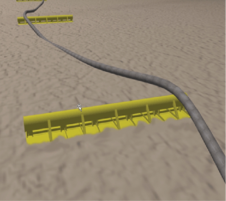
It shall be noted that such devices may create slugging phenomena when the pipeline transports multiphasic fluid inducing fatigue in the line.
Pre-Bent Pipe (R&D)
The Fairway Field development in Mobile Bay was installed in 1991. The pipeline employed was a 6-inch CRA lined (mechanically bonded) pipe (*). Each pipe joint was bent onshore into an 8 degree bend and then welded into double joints. The pipe was S-layed in shallow water using a modified firing line; a lay rate of 0.5 km/day was achieved (**). The pipeline was trenched. The aim of this approach is not really to develop lateral buckling; rather the pipe expands laterally at each joint, absorbing the thermal expansion as an axial spring would. However, in principle the approach could be modified so that the pre-bent joints are spaced less frequently and act as buckle initiators in the same way as the snake lay model.
(*) Mobile Bay Fairway Field Flowline Project. Lanan, G and Barry, D. OTC 7014, 1992.
(**) Theory and Practise of Installing Pipelines by the Pre-Snaking Method. Vermeulen, H.R. International Offshore and Polar Engineering Conference. IOPE 1995.
The in-line accumulator (ILA) system can be distributed along the pipeline at regular spacing to absorb ends expansion (up to 4m) and mitigate any lateral buckling, applying an initial pretension of the ILA system (onshore). The configuration of the ILA System is depicted in the Figure 2.19, “ILA Main Characteristics”:
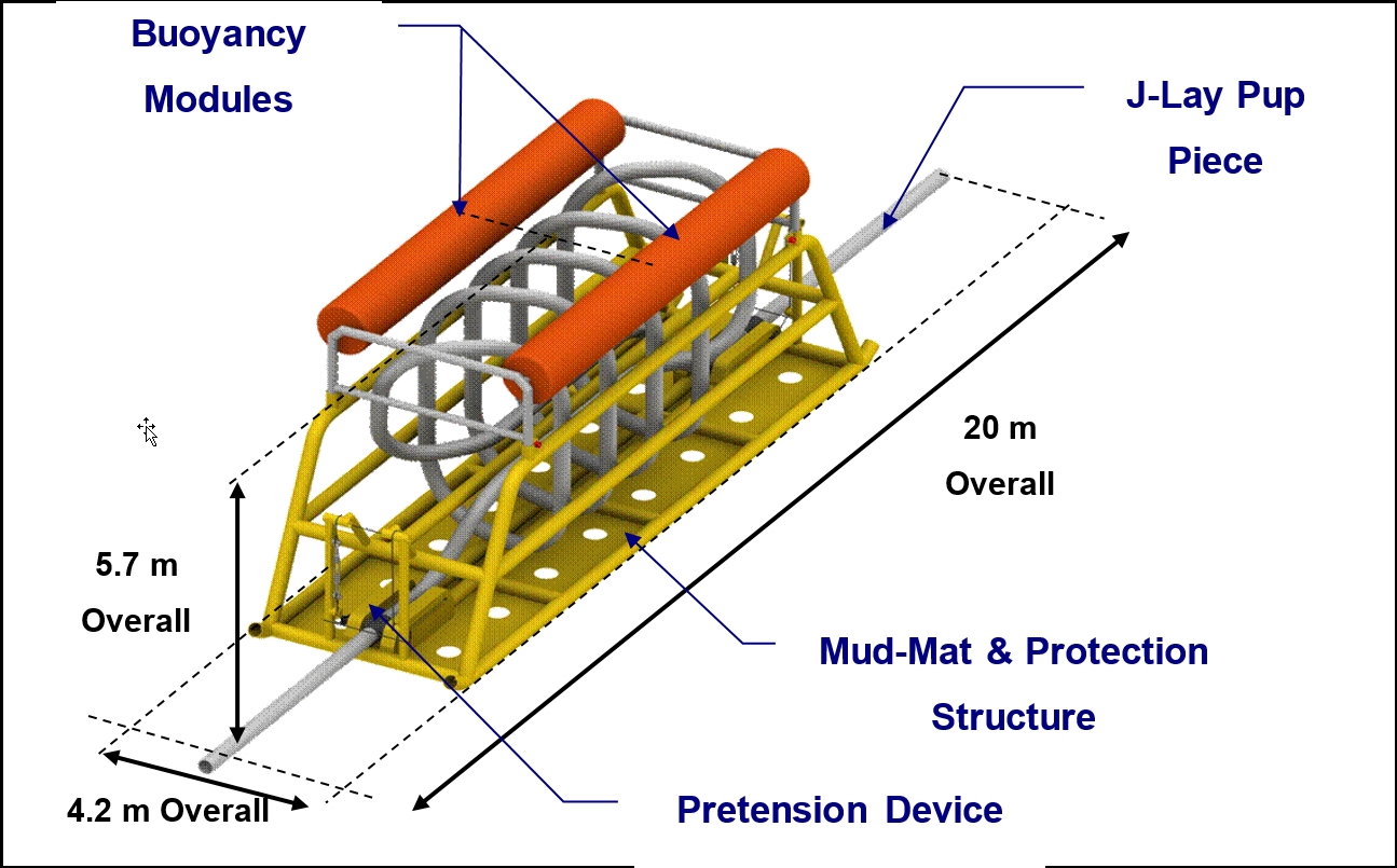
2.3.8 Protection
External interference of pipelines, for which protection may be provided, generally fall into two categories, namely dropped objects and trawling. Regionally, other sources of damage may exist such as iceberg scour. This section considers the sources of potential damage and the methods of protection typically adopted.
Dropped Objects
Dropped objects are a potential hazard in the vicinity of installations, or where vessels are working over or close to flowlines. The area of risk from dropped objects is localised and therefore protection measures are also localised. The DNVGL-RP-F107 guideline provides a useful reference for the evaluation of dropped object loads and acceptance criteria to pipeline (including polymer and concrete coating).
Typical sources for dropped objects are platform or installation supply, and drilling and work-over, where typical dropped objects could include containers, drill pipe, scaffold pole, drill collar, BOP stack, etc. Examples of typical tubular and bulk items that may be considered in dropped object protection design are shown in Table 2.5, “Typical tubular dropped objects” and Table 2.6, “Typical bulky dropped objects”. The design cases are, however, job specific and these are shown for illustration only.
Table 2.5 - Typical tubular dropped objects
Object | WT | L | Mass | |
Drill collar | 280mm | 102mm | 9450mm | 4.2Te |
Scaffold pole | 48mm | 4.5mm | 6400mm | 31kg |
Drill casing | 760mm | 9.5mm | 13100mm | 2.3Te |
Table 2.6 - Typical bulky dropped objects
Object | L | B | H | Mass |
Container | 6100mm | 2400mm | 1200mm | 15Te |
Skid-mounted generator | 5250mm | 1910mm | 2950mm | 10kg |
BOP | 540mm (OD) | 1820mm (Width) | 1850mm | 20.6Te |
An object dropped through water will, due to hydrodynamic effects, travel laterally as well as vertically. The area of seabed over which an object may impact will increase with increasing water depth. The impact risk for a pipeline on the seabed therefore generally reduces with increasing water depth. Consequently, dropped object protection is not normally specified in deep water applications, although is often required in water depths typical of the North Sea.
Dropped Object Protection
Dropped object protection can be provided by a number of methods. Methods commonly used include mattresses, rock-dump, tunnels and trenching. Mattresses are made up of concrete blocks strung together on polypropylene rope. Depending on the configuration of the concrete segments, they may flex in either 1 or 2 planes and can be made in a large range of sizes. The main design issues for mattresses when used for protection are penetration resistance, concrete integrity under impact (i.e. spalling and scabbing of concrete), distribution of impact load, hydrodynamic stability, installation loads and accuracy of placement. Installation is usually from a DSV or MSV.
Rock-dump can be accurately deployed over the pipe to provide a protective berm. The main design considerations for rock-dump are the protection afforded by the rock dump and the stability and long term integrity of the rock berm. In determining the protection one is specifically ensuring that there is a sufficient depth of cover over the top of the pipe to ensure that dropped objects cannot penetrate through to the pipe, and that loads are dissipated effectively. The long term stability of the berm is ensured by defining the angle of the berm sides and the size of rock, to ensure that rock does not dissipate under the effects of environmental/hydrodynamic loading.
For localised areas where movement of the pipe is not to be restricted, such as at spool-pieces, tunnels can be used. These may be of either concrete or steel construction and are normally of a gravity based design. The main design issues for tunnels are hydrodynamic stability, material, installation loads, penetration resistant, energy dissipation, lateral displacement, foundations and installation accuracy. There are often safety and other operational issues with the installation of tunnels.
As with all aspects of pipeline design the practicalities of any methodology must be considered carefully by consulting operations personnel.
Trawling
Historically, trawling has tended to be an issue in European waters only, where fishing practices involve the use of heavy on-bottom gear. However, similar practices are adopted elsewhere around the world and trawling may be of significance in other regions. There are two guidelines available for assessing the consequences of trawl gear interaction on pipelines, namely:
- HSE OTH561 - Guidelines for trenching design of submarine pipelines;
- DNVGL-RP-F111 – Interference between Trawl Gear and Pipelines.
Demersal trawling is widespread and intense around European waters. The demersal trawling activities that could interact with a pipeline would be either:
- Beam trawling: employed for the capture of flat fish and using a steel beam to hold the net open. A skid-like shoe assembly holds the beam off the seabed at each end.
- Otter trawling: employed for the capture of round fish with the net being held open by two otter boards which use a combination hydrodynamic force and friction with the seabed to create a spreading force on the mouth of the net. Otter trawling may also employ a central clump weight if two nets are being towed by a single vessel, i.e. twin-rig otter trawling.
Other regions of the world may employ these practices and trawling interaction could therefore be of significance. A review of fishing practices in the region of a pipeline is therefore essential in order to determine the protection requirements.
The design for trawl gear interaction considers two load scenarios:
- Impact of the gear in the pipeline;
- A transient load as the gear is dragged over the pipeline.
A third load scenario may also be considered, a sustained load due to hooking of the gear beneath the pipeline.
The impact design considers a transfer of kinetic energy from the gear to the pipeline. Both design guidelines consider empirical relationships for how much energy is dissipated through local Deformation of the pipe wall, i.e. denting, and how much is dissipated globally. A finite elements based methodology is also outlined in OTH561. The denting response is again defined by analytical models. Both guidelines base their dent response models on that proposed by Ellinas and Walker, as shown below. The DNVGL-RP-F111 model is a modified version of this simple equation.

Ellinas, CP and Walker, AC, Effects of Damage on Offshore Tubular Bracing Members, International Association of Bridge & Structural Engineers: Colloquium on Ship Collision with Bridges and Offshore Structures, Copenhagen, 1983.
di is the dent depth;
Dm is mean diameter of pipe;
E is impact energy;
σy is the yield stress of the pipe;
t is the nominal wall thickness.
Evaluation of the effects of pullover is performed by FE analysis. Both DNVGL-RP-F111 and OTH561 define the requirements of the analysis. The pullover loads are specified in the DNVGL guideline and the OTH561 defines an analytical method by which the force-time load history can be calculated.
Similarly, the effects of hooking are determined by FE analysis.
Trawling Protection
There are two main methods by which protection against trawling is provided. Firstly, thick pipeline coatings can protect against the impact loading. The following conservative guidelines may be used as a first pass on trawl gear impact protection.
Protection against trawl gear impact is provided by:
- Concrete coating;
- Thick insulation coating (thickness > 20mm for otter trawls; thickness > 45mm for beam trawls).
The second method of protection against trawl gear is trenching of the pipeline. Lowering the pipeline below the level of the seabed greatly reduces potential impact and pullover loadings and increases the resistance to movement of the pipeline. Backfill of the pipeline trench will provide full protection against trawl interaction.
Other
Other sources of pipeline interaction may be encountered. One of the main other source of pipeline damage may be the slippage of other barge anchor, inducing a hooking of the line. Clearance with pipelines based on local regulations and/or international standard and/or Total Specifications shall be followed. Another source is the iceberg scour in Newfoundland where conventional protection methods described above are ineffective. The protection measures for very high design load cases such as iceberg scour consist of a contingency for flushing of the line and replacement of repair of the damaged section if the pipeline is struck.
2.3.9 Cathodic Protection
Cathodic protection is used with anti-corrosion coatings, to provide corrosion protection to the external surface of the pipeline. Protection is achieved by making the pipeline the cathode in an electrochemical cell. Cathodic protection systems for subsea pipelines normally utilise sacrificial anodes and this is the method briefly described within this section.
Detailed guidance on the design of sacrificial anode cathodic protection systems is provided in the DNVGL Recommended Practice RP-F103.
Principle of Design
The basic electrochemical process of spontaneous corrosion of steel in water is illustrated in Figure 2.20, “Illustration of the steel corrosion process”. Both anodic and cathodic sites are produced on the surface of the steel forming an electrochemical cell. The iron atoms dissolve from the surface of the steel at anodic sites to produce ferrous ions in solution. The resultant electrons migrate through the steel to cathodic sites, where they react with oxygen and water molecules to produce hydroxyl ions.
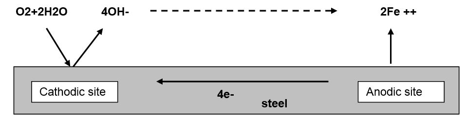
The basic principle of the cathodic protection system is to supply a sufficient current to the surface of the steel to fully satisfy the electron demands of the cathodic reaction thereby eliminating the anodic reaction on the steel surface. This is achieved by connecting a dissimilar metal to the pipeline with the seawater, which will corrode preferentially, thereby forming a galvanic cell as illustrated in Figure 2.21, “Galvanic cell formed by zinc sacrificial anode”.
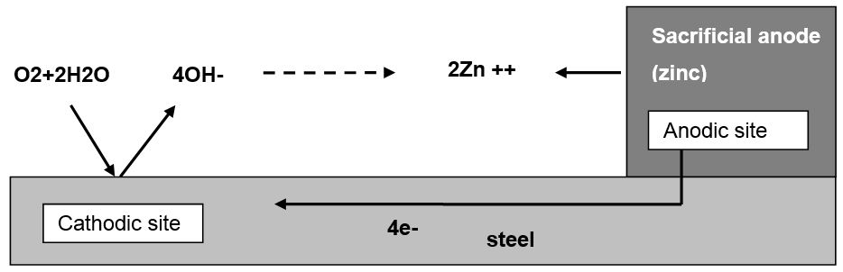
The sacrificial anode must have a surface potential that is more negative than that of steel in order that it becomes the anode in the reaction. This means that the anode material should be less noble than iron. Materials typically used in pipeline sacrificial anodes include zinc or aluminium as the base material.
In designing the anodes there are three basic requirements to satisfy:
|
Current Output Requirements
The current density required to protect exposed steel will vary with geographical location and water depth. The required current density will also increase with increasing pipeline operating temperature. The required current increases in colder climates and reduces with increasing water depth. DNVGL-RP-F103 defines design current densities for tropical, sub-tropical, temperate and arctic environments and for water depths of less than 30m and greater than 30m. DNVGL-RP-F103 also provides corrections to current density when the operating conditions will take the steel surface temperature above 25°C. For water depths greater than 300m refer to deepwater considerations, NACE publication 7L192, Cathodic Protection Design Considerations for Deep Water Structures, 1992.
Design current density requirements reduce through the life of the pipeline due to the build-up of protective scale on the exposed surface of the steel. However, the area of steel exposed due to breakdown of coatings will increase through the life, normally resulting in a greater overall current demand at the end of the pipeline life. DNVGL-RP-F103 provides conservative guidance on coating breakdown rates for use in the design.
The initial coating breakdown will depend not only on the coating quality but also on the field coating philosophy. In the North Sea it is normal practice to apply field joint coating. In other areas of the world field joints may be left uncoated; when this is the case, the exposed area of the field joints must be accounted for in the initial coating breakdown assessment.
The current capacity of the anode is a function of its surface area. With the bracelet anodes typically employed on pipelines, the anode surface area decreases as it is consumed and therefore the end of life surface area together with the end of life current demand normally gives the governing current output requirement condition.
Anode Mass Requirement
The anode mass requirement depends on the rate at which the anode is consumed throughout the life of the pipeline. This depends on the mean current density requirements, the average coating breakdown during the pipeline life and the current capacity of the anode material. Again, DNVGL-RP-F103 provides design criteria for mean current density requirements and mean coating breakdown rates.
Attenuation Requirements
In most practical circumstances, the attenuation requirement does not govern the anode design. In order to avoid issues of anodes being spaced too far apart to adequately protect the pipeline RP-F103 specifies a maximum anode spacing of 300m. For larger distances than 300m (i.e. by design), the effect of the metallic resistance in the pipe wall will be taken into account. The calculation of the maximum anode distance to provide sufficient anode current output is detailed in DNV RP F103.
Practical Requirements
Pipeline anodes are normally in the form of half-shells clamped around the pipe. On reeled pipe, the anodes have tapered ends to assist their movement over the rollers on the vessel ramp. Each half shell is electrically bonded to the pipe using a copper bonding strap. This is attached to the pipe surface using brazing welding.
Size Considerations
Anodes can be manufactured in thickness varying from about 30mm minimum up to 125mm maximum. On the reel barge, the anodes are installed on the ramp after the straighteners and tensioners, and have to be man-handled into position. There are therefore practical handling constraints which limit the anode length to 1m maximum and the mass to 100kg maximum.
Over Protection
Cathodic protection will be accompanied by the formation of hydroxyl ions and hydrogen at the surface of the steel. These products can cause disbondment of the coating and stress corrosion cracking of susceptible materials. The designer should consider the implications of overprotection of the pipe. Cathodic disbondment can be avoided by ensuring that protective potential is never more negative than –1.1V. The use of aluminium or zinc anodes avoids this problem.
In general, steel and non-ferrous alloys with yield strengths of up to 550 MPa are considered compatible with cathodic protection systems utilising zinc or aluminium anodes. However, higher strength materials can be used provided CP design eliminates the potential causes of hydrogen embrittlement. The DNV RP F112 (draft available) gives detailed recommendations on characteristic load effects and acceptance criteria that need to be considered in the design of subsea systems where 22Cr and 25Cr duplex stainless steels will be used in conjunction with cathodic protection.
2.3.10 Pipe Free Span Calculations
The design for pipeline freespans is defined in a number of guideline documents, including:
DNV Classification Note 30.5, Environmental conditions and environmental loads, March 2000;
DNV RP-F105, Free spanning pipelines, February 2006;
Of the available guidelines, the methods specified in DNV Recommended practice RP-F105 are recommended.
Span Issues and Criteria
There are three basic issues considered in span criteria:
Bending, due to hydrodynamic loads and self weight;
Global buckling, due to axial compressive loads resulting from temperature and pressure;
Fatigue due to vortex induced vibrations.
A further issue that is now considered within the North Sea is the interaction of fishing gear on pipelines and the consequential risk that a span may present to a fishing vessel.
Bending
The normal industry criteria set for bending is that stresses should not exceed code allowable limits for installation, hydrotest and operations. The allowable stress limits vary from one code to another and therefore small variations in these criteria will exist depending on the code used. This philosophy is intrinsically based on allowable stress design codes. DNV’s recommended practice RP-F105 ‘Free Spanning Pipelines’ is based on the limit state approach adopted in the pipeline code DNV OS-F101 and sets criteria based on local buckling.
Global Buckling
The common criterion for global buckling, again widely used throughout the industry, is to set a limiting span length such that a global buckle (calculated using Euler buckling formula) is avoided. The axial compressive load on the span is a function of the operating temperature and pressure and the residual lay tension. DNV’s approach does not consider global buckling as a separate event but addresses the response to axial loading within the bending response and criteria.
Vortex Induced Vibrations
Flow past a spanning pipeline will induce vortex shedding from the pipe. This can initiate vibrations in the pipe which can lead to fatigue damage. It is in the treatment of vortex induced vibrations that one can see the main differences in span criteria. The approaches seen include:
|
The VIV criteria employed tends in many cases to be dependent on whether the pipeline is under construction or in operation. During the construction phase the criteria has traditionally been set to avoid vibrations. We have seen both in-line vibrations and cross-flow vibrations being used as the limit. During operation, the general philosophy is to determine the remaining fatigue life of the span and ensure that it will be fit for the remaining service life. In determining remaining fatigue life other contributing fatigue sources such as wave and tidal cycles are considered.
Trawling Interaction
In the North Sea, the interaction of trawling with pipelines is now considered in operational span criteria. Whilst not specified in the design methods listed above, there is a requirement on UK pipeline operators to report potentially dangerous spans. This is as a result of an incident when a trawler caught its gear beneath a high span and subsequently capsized and sunk with the loss of the crew. The criterions is set on span height rather than span length and introduces requirements for reporting of spans so that they can be marked on Admiralty charts. This is not normally considered as a design requirement.
Design Approach
The design approach normally differs between the design stage and the operational stage. Often at the design stage, before the pipeline is installed, the designer is looking to identify anomaly limits, i.e. span lengths at which problems could arise. Following construction or during operation, once spans have been identified the approach is usually to define the fitness-for purpose of an actual span. The basic approaches to each aspect of the span design are outlined in the following.
Stress
The stress check considers the extreme environmental loadings on the span, assesses resultant bending and determines and checks the resultant combined stresses against code allowable limits.
DNV RP-F105 uses the limit state design approach of DNV OS-F101. This combined load check is therefore based on ultimate limit state (ULS) criterion rather than allowable stress. The recommended practice defines the procedure for determining the maximum resultant static and dynamic responses of the span to both direct wave action and vortex induced vibrations (VIV). The responses are combined and a check against the ULS criterion on local buckling is performed. The local buckling criterion is taken from DNV OS-F101.
Global Buckling
Checks on global buckling using Euler strut buckling criteria are sometimes performed. The effective axial compressive force in the pipeline must be less than the critical load for strut buckling of the spanning pipeline. The critical axial load for strut buckling Pcr is given by:
![]()
Where:
E is the elastic modulus of the linepipe steel;
I is the second moment of area of the pipe section;
L is the span length;
C is a factor defined by the span end conditions as follows;
C = 1 pin-pin;
C = 2 pin-fix;
C = 4 fix-fix.
The tensile effective axial force is given by:
![]()
Where:
Heff is residual lay tension;
Δpi is internal pressure difference relative to as laid;
Ai is internal cross-sectional area;
ν is Poisson’s ratio;
As cross-sectional area of steel;
α Coefficient of expansion;
ΔT temperature difference relative to as laid.
DNV RP-F105 does not include a separate global buckling check, as the effects of axial compressive load are accounted for in the static deflection model and therefore considered in the ULS local buckling criterion described above.
Vortex Induced Vibrations
As water flows past the pipeline span, vortices are shed in the wake. The vortices are shed periodically at a frequency governed by the flow velocity. As the vortices are shed the pressure distribution around the pipe circumferences fluctuates producing oscillating loads on the span. Under flow conditions where the shedding frequency of the vortices is close to the natural frequency of the span the amplitude of resultant motion increases significantly and periodic motion locks-in. These vortex induced vibrations (VIV) may result in fatigue damage.
With increasing velocity, the vibration of the span passes through a number of oscillation modes. At lower flow velocities, the vortices are shed symmetrically from top and bottom of the pipe, giving an in-line oscillation mode (oscillations in-line with the direction of current flow). At increased velocity, the vortices are shed asymmetrically, giving initially a further mode of in-line oscillation and then a cross-flow mode (oscillations across the flow direction). The design guidelines use empirically derived response curves to define the amplitude of motion under specific flow conditions. The response is defined in terms of a number of dimensionless parameters, namely:
Reduced velocity;

Keulegan-Carpenter number;

Current flow ratio;

Stability parameter;

In these equations:
Uc is the current induced water particle velocity normal to the pipe;
Uw is the wave induced water particle velocity normal to the pipe;
fo is the pipeline span natural frequency;
fw is the wave frequency;
me is the effective mass per unit length = pipe mass + added mass of water;
D is the hydrodynamic diameter, i.e. overall outside diameter;
ζT is the total modal damping ratio at a given vibration mode comprising: structural damping + soils damping + hydrodynamic damping
As a first pass the following values may be used, although it is recommended that reference be made to RP-F105 for detailed guidance, structural damping (=0.005 first pass), soils damping (=0.01 first pass), hydrodynamic damping (=0.0 first pass);
ρ is the seawater density.
Approximate analytical models or finite element analysis can be used to define natural frequency and stress response of the span.
The fatigue damage due to VIV can be determined for a specific wave and current combination. By considering all wave and current combinations, the probabilities of occurrence and the frequencies of oscillation the total fatigue damage can be assessed. Oscillations in directions both in the line of flow (in-line) and across the line of flow (Cross-flow) need to be assessed.
The basic procedure is illustrated in Figure 2.22, “Flow chart over design checks for a free span”.